Introduction

The aerodynamic shape optimization consists of an iterative procedure, wherein the flow field around (or inside) each candidate solution has to be computed several times (once for each candidate solution). Aiming to obtain the approximate solutions of the governing flow Partial Differential Equations (PDEs), it is necessary to apply the proper domain discretization on which the PDEs will be locally solved. In such an optimization framework, the utilized (structured or unstructured) grid should be either re-generated for each candidate geometry, or an initial grid is deformed along with the deformation of an initial (reference) geometry. The latter approach saves a lot of computational resources, especially when the PDEs solution for a previous geometry can be imposed as an initial condition for the initialization of the simulation of a following geometry. Given the importance of grid adaptation (mesh deformation or mesh morphing) techniques, over the latest years, several methodologies have been proposed, aiming to reduce the required computational time, while enhancing the quality of the resulting meshes. Such methodologies are based on the Radial Basis Functions (RBF) interpolation, Free-form Deformation (FFD), algebraic methods, as well as physical analogies and PDE methods (Samareh, 1999; Zhao and Forhad, 2003; Selim and Koomullil, 2016; Leloudas et al., 2018; Gagliardi and Giannakoglou, 2019; Leloudas et al., 2020).

One of the promising methods for mesh and geometry deformation is the use of harmonic coordinates. Harmonic coordinates were originally introduced by Pixar Animation Studios for character articulation. Based on mean-value coordinates proposed by (Floater, 2003), the harmonic functions (solutions to the Laplace’s equation) applied on closed triangular meshes (cages), as presented in the work of (Ju et al., 2005), were originally used for object articulation, by introducing a cage/object coordinate system; however, their coordinates failed to be non-negative. Joshi et al. (2007) introduced the harmonic coordinates for object deformation, and showed that these are non-negative and have interior locality, as a result from the fact that harmonic coordinates are solutions to the Laplace’s equation. They were also emphasized the benefits of cage-based approach for object articulation, compared to Free-form Deformation (FFD). In the cage-based approach the cage is manually deformed and the contained object is automatically deformed. This is a decoupled procedure, which allows for the deformation of objects consisting of many primitives, and additionally the deformations can be automatically transferred form low-detailed to high-detailed versions of the object to be deformed.

In this work, a modification to the classical harmonic coordinates’ concept is introduced for the deformation of 2D geometries (and the corresponding computational mesh) for aerodynamic shape optimization purposes. The 2D geometries to be optimized are defined as closed periodic B-spline curves (Piegl and Tiller, 1995). In the classic methodology of (Joshi et al., 2007) the functions used as boundary conditions for the numerical solutions of the Laplace’s equation (to produce the harmonic functions) are linear B-spline basis functions applied on a piecewise linear boundary (cage), which encloses the geometry to be deformed. In the proposed methodology the functions used as boundary conditions can be non-linear B-spline basis functions, applied on a non-linear boundary (the B-spline curve of the boundary). Actually, the B-spline basis functions of the corresponding boundary B-spline curve are used as harmonic functions along the mesh boundary, coinciding with the geometry to be deformed (the B-spline curve). Thus, any deformation to the B-spline boundary, through the movement of the curve’s control points, can be successfully propagated to the interior of the computational domain, resulting in the concurrent and conformable modification of the B-spline boundary and the entire computational mesh. The main advantage of this approach is that the utilized cage is the control polygon of the B-spline boundary (or boundaries) of the meshed domain and the deformed boundary is still a parametric B-spline curve. This is a valuable characteristic for design optimization methodologies, as the final (optimized) geometry automatically results in a parametric form.

For the computation of the harmonic coordinates a node-centered Finite-Volume based solver for unstructured meshes is used, which is enhanced with an agglomeration multigrid scheme, so as to reduce the computational burden (the main drawback of the methodology).

Methodology

A pth degree B-spline parametric curve is defined as (Piegl and Tiller, 1995):

where the {Pi} are the n+1 control points and the {N_i,p(u)} are the p^th-degree B-spline basis functions, while u being the parameter of the parametric curve, taking values in the interval [a,b].

We use the B-spline curve to define one (or more) of the boundaries ϑΩj of a 2D computational domain Ω∈R2 (Figure 1). This boundary could be an internal (usually) or external one, the other boundaries being fixed during the optimization procedure and defined with different types of lines. In general, more than one B-spline boundaries can be modified during an optimization procedure, using the proposed methodology. We aim to develop a computational methodology, which allows for the concurrent and conforming deformation of the B-spline boundary, and the corresponding computational domain (i.e., the contained computational grids), by simply moving only the B-spline control points Pi (without using any additional polygonal cage). Moreover, the grid used for the solution of the flow PDEs could be the same with the one used for the successive solutions of the Laplace’s equation (used to produce the harmonic functions).

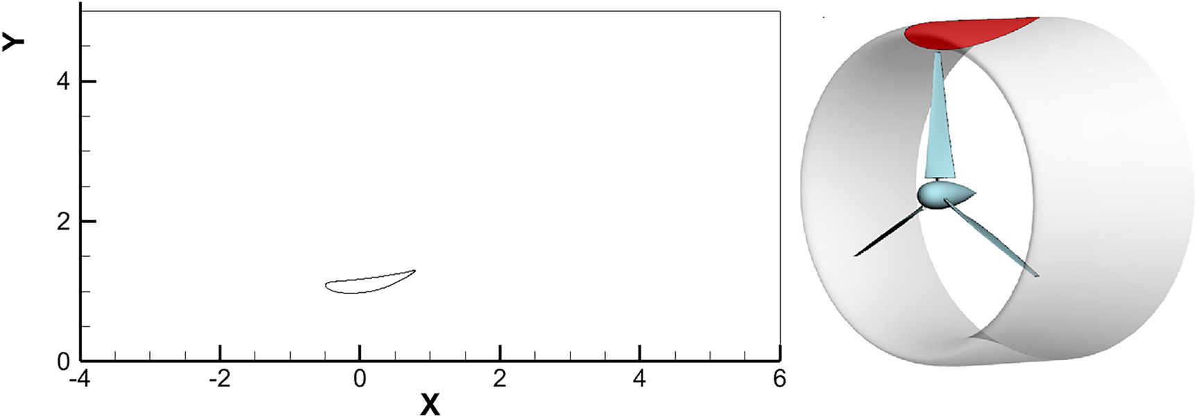
Figure 1.

(Left) A computational domain Ω for the flow simulation around a generic axisymmetric diffuser, used in a Diffuser Augmented Wind Turbine. X-axis is the axis-of-symmetry of the diffuser. The 2D geometry of the diffuser is defined using a single 3rd-order B-spline curve, with 11 control points. (Right) A Diffuser Augmented Wind Turbine (schematic).

The displacement vector ΔC(u) of a discrete point on the B-spline curve (corresponding to a parameter value u) can be computed as a function of the displacement vectors ΔPi of all the n+1 control points Pi,i=0,…,n. If C0(u) is the initial position of the discrete curve point corresponding to parameter u, C1(u) is its final position, Pi0 and Pi1 are the initial and final positions of the B-spline control points, then the calculation of ΔC(u) can be made as follows:

where

Therefore, the displacement vector ΔC(u) of a discrete point on the B-spline resulted as a function of the displacement vectors ΔPi of all the n+1 control points Pi. Let us now define n+1 harmonic functions Fi,i=0,…,n inside the initial computational domain Ω (Figure 1), each one of which results as the solution to the Laplace’s equation ΔFi(r)=∇2Fi(r)=0 inside the initial computational domain, r being the position vector for each point inside the domain, with the (Dirichlet) boundary conditions defined on the (curved) B-spline boundary as:

and Fi=0 in all the remaining (non-deformed) boundaries. Thus, the boundary conditions are defined only for the B-spline boundaries to be deformed, and not for the remaining (non-deformed) boundaries of the computational domain; because the harmonic coordinates are defined using the displacement vectors ΔPi of all the n+1 control points Pi and not the control points Pi themselves (contrary to the classical methodology).

We construct an unstructured mesh inside the computational domain (consisting of triangular or triangular/quadrilateral elements), the B-spline curve being one of the boundaries of the domain (using the discrete points C0(ul) on the B-spline boundary as boundary grid nodes) (Figure 2). For our illustrating example, the discrete solution (harmonic function) F~3 (resulting from the solution of the Laplace’s equation in the corresponding domain by using Basis Function N3,3(u) as boundary condition), is depicted in Figure 3.

Figure 2.

An unstructured mesh, consisting of triangular elements, to be used for the numerical solution of the Laplace’s equation for n+1 times, to compute the corresponding Harmonic functions.

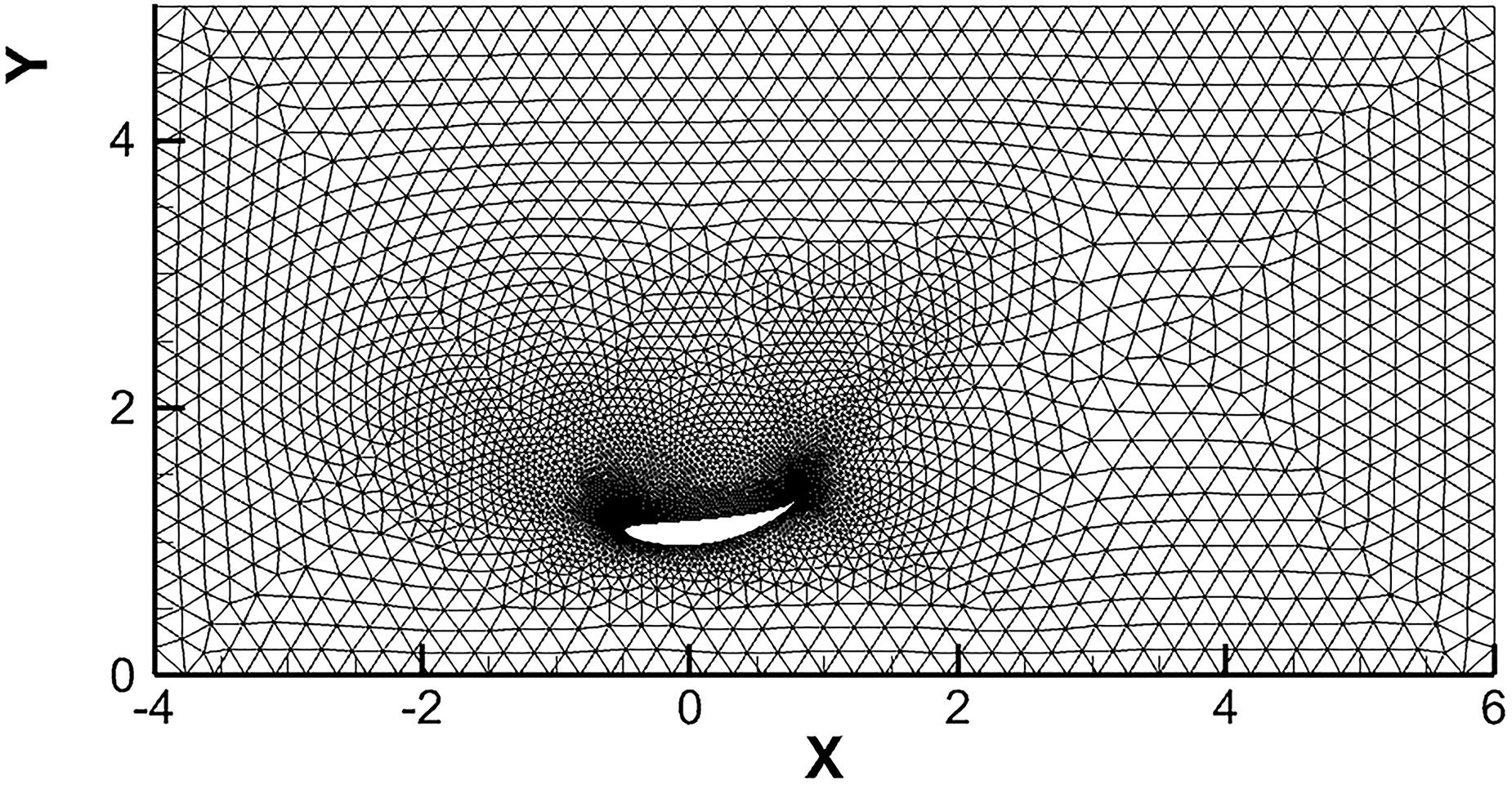
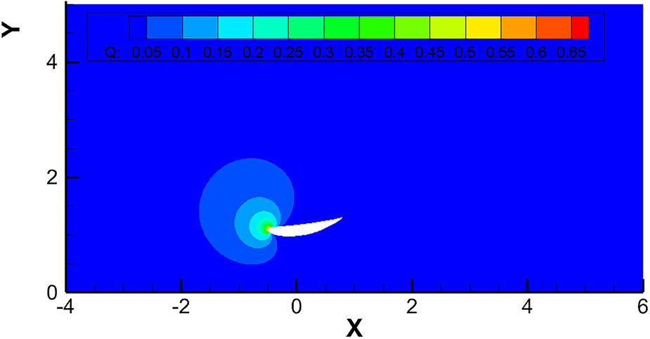
Figure 3.

The discrete solution F~3, which resulted for the Basis Function N3,3(u), applied as a Dirichlet boundary condition on the B-spline boundary of the computational domain.

Having all the discrete solutions F~i of the Laplace’s equation (harmonic functions), computed for each different set of (Dirichlet) boundary conditions, we can use them to interpolate inside the computational domain discrete movements applied on the control points of the boundary B-spline curve, as:

where r is the position vector for each point inside the computational domain.

However, by construction, the discrete solution F~i on a discrete point C0(ul) belonging to the B-spline boundary has the value of the corresponding basis function N_i,p(u_l). Therefore, the previous summation (Equation 5), for a boundary point C0(ul) becomes:

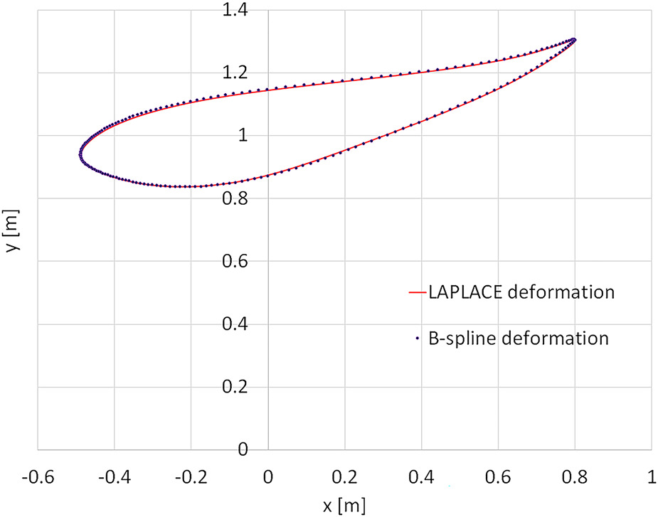
We, thus, proved that the displacement of the discrete points on the B-spline boundary, resulting from the application of the harmonic coordinates are exactly identical to the displacement resulting from the corresponding B-spline procedure (Equation 2). Therefore, the proposed procedure can be used to concurrently and conformably deform the B-spline boundary and the internal computational grid inside the computational domain. It has to be emphasized here that the application of the B-spline displacement procedure is not required and only the basis functions are needed for the procedure (to define the corresponding Dirichlet boundary conditions for the consecutive solution of the Laplace’s equation). Figure 4 provides a comparison between the displaced boundary, computed using the harmonic coordinates procedure and the B-spline procedure (3 control points have been displaced in this example). As it can be seen, the results are identical. Figure 5 contains the initial and the deformed grids, resulted for the airfoil deformation of Figure 4.

Figure 4.

The result on the shape of the boundary of the displacement of 3 B-spline control points, as computed using the B-spline procedure and the Harmonic Functions procedure.

Figure 5.

The initial and the deformed grids, resulted for the boundary deformation of Figure 4.

At this point, it should be mentioned that the proposed procedure is not applicable only to mesh morphing and design optimization, but has potentially many applications, such as in computer graphics. A major difference of the proposed methodology, compared to the classic methodology of morphing through the use of harmonic coordinates (Joshi et al., 2007), is that in the proposed methodology the harmonic functions are combined with the displacement vectors of the control points of the deformed B-spline boundary, while in the classic methodology the harmonic functions are combined with the position vectors of the control points of a separate cage. This fundamental difference allows for the proposed methodology to be applied directly to curved boundaries, while the original methodology can be applied solely on the linear boundaries of the cage.

A different and denser computational grid (to be used for the solution of the flow equations) can be deformed through the proposed methodology, by simply interpolating the computed harmonic functions from the coarse grid to the fine one. Alternatively, the Laplace’s equation can be solved directly to the final computational grid, with higher computational cost; however, this cost is spent once at the beginning of the optimization procedure.

Numerical solution of the Laplace’s equation

Laplace’s PDE, providing the harmonic functions as its solutions, can be written in its simplest formulation as follows (Svard and Nordstrom, 2004):

where scalar function F(x,y) denotes a solution to the problem. Adding a temporal term, allowing for the prediction of unsteady conditions, and using the flux terms G and H, namely the derivatives of F in x and y directions, respectively (G=∂F/∂x,H=∂F/∂y), it can be expressed with a differential time-dependent form as (Nikolos and Delis, 2009; Lygidakis et al., 2016):

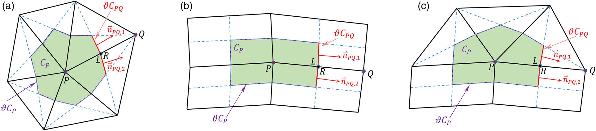
For the spatial discretization of the aforementioned PDE, a node-centered Finite-Volume (FV) scheme is employed along with two-dimensional unstructured grids, composed of triangular and/or quadrilateral primary elements. The corresponding median dual control volume of each mesh point (node) is defined by the lines connecting edge midpoints and the barycenters of the primary elements sharing this node (Lygidakis et al., 2016; Leloudas et al., 2020). Figure 6 depicts examples of such control volumes, comprised of (a) only triangular elements, (b) only quadrilateral ones, and (c) both triangular and quadrilateral ones. ∂CPQ is the shared part of ∂CP and ∂CQ; the latter denote the boundaries of the control volumes CP and CQ (of nodes P and Q, respectively). Considering the aforementioned discretization, Equation 8 is integrated over the control volume CP of each grid node P and subsequently transformed as:

Figure 6.

Control cell examples, composed of different type of faces.

where EP is the area of the control cell CP around node P and KN(P) is the set of its adjacent nodes, each of them denoted with Q and connected to P with an edge PQ (Nikolos and Delis, 2009; Delis et al., 2011). Finally, fPQ stands for the fluxes going through the interface ∂CPQ, computed via the following expression:

where n→PQ=n→PQ,1+n→PQ,2 is the outward normal vector to ∂CPQ; nPQ,x and nPQ,y denote its components in x and y directions, respectively.

For the aforementioned calculation the gradients of F have to be obtained previously at edge’s endpoints. This is succeeded with an element-based approach, considering the construction of a new control volume for each grid node, composed by all its neighbouring facets (Barth, 1992; Nikolos and Delis, 2009; Delis et al., 2011; Lygidakis et al., 2016). Figure 7 illustrates examples of such control volumes, constructed by quadrilateral and triangular elements. Considering these new control cells, the required nodal gradients are computed using the Green-Gauss theorem via an edge-based formulation (Barth, 1992). Ultimately, utilizing the edge-based data structure of the proposed algorithm the fluxes of Equation 9 are obtained with a single edge-loop, as no information is needed about the cell topology (Kallinderis and Ahn, 2005; Lygidakis et al., 2016; Leloudas et al., 2020).

Figure 7.

Control cells used for the computation of nodal gradients.

Appropriate boundary conditions are implemented as well, either by contributing proper values to the fluxes’ sum on boundary nodes (Von Neumann conditions) or defining explicitly their values of function F (Dirichlet conditions) (Lygidakis et al., 2016; Leloudas et al., 2020).

Since the aforementioned flux calculations have been accomplished for each computational node, Equation 9 for a node P is reformulated as follows (Lygidakis et al., 2016; Leloudas et al., 2020):

where ΔFPn+1 denotes the correction of F on node P at time step n+1. Analogously, R→Pn stands for the fluxes’ sum at the previous time step n and ΔtP for the time step of the iterative procedure. The latter is calculated for each node with a local time-stepping methodology as:

where CFL is the Courant-Friedrichs-Lewy number and l_minedge,P is the length of the shortest edge connected with the examined node P. This acceleration technique allows for the maximum permissible time step to be employed for each node and consequently to improve the convergence rate of the relaxation procedure (Blazek, 2001). Finally, the corrections to F are computed iteratively implementing (at each external time step) the explicit second-order four-stage Runge-Kutta method (RK(4)) (Lallemand, 1988), hence gradually approximating the final steady state.

The numerical solver is enhanced with an agglomeration multigrid scheme to further accelerate the solution procedure, especially in large-scale problems (Blazek, 2001; Nishikawa et al., 2010; Lygidakis et al., 2016). Although this approach was initially introduced in a three-dimensional CFD solver (Lygidakis et al., 2016), it was incorporated in the current two-dimensional Laplacian algorithm in an almost straightforward manner, mainly due to its edge-based formulation. In accordance to this scheme, the final solution is relaxed on a set of successively coarser grids, in order the low-frequency errors to become high-frequency ones and consequently be damped more efficiently. The generation of each coarser mesh, composed of irregular polyhedral cells, is succeeded by merging the adjacent control volumes of the finer grid, isotropically or directionally (either selected by the user). The merging process begins from the boundary nodes following pre-defined rules and extends gradually to the interior domain, resembling in that way the advancing-front technique. In case of hybrid grids, including both quadrilateral and triangular elements, it is accomplished firstly at quadrilateral areas, usually located at boundaries. The aforementioned agglomeration procedure is repeated until the required set of successive coarser grids is achieved; a number of four or five levels is usually adequate. The multigrid accelerated solution is obtained with the Full Approximation Scheme (FAS) in a V-cycle process. According to this methodology Equation 11 is solved only at the initial finest mesh, whereas at the coarser ones, approximate formulations of it are relaxed (Blazek, 2001; Nishikawa et al., 2010). The interaction between each two successive spatial levels is achieved via the restriction of F values and flux balances, computed at the centres of control cells, from the finer to the coarser resolution, as well as with the prolongation of the corresponding updated corrections to F from the coarser to the finer one. The proposed algorithm can be further accelerated with a combined (Full Multigrid) FMG/FAS method, according to which the whole procedure begins from the coarsest grid and, as the number of iterative cycles increases, it extends gradually to the finer meshes up to the initial finest one (Lygidakis et al., 2016).

Results and discussion

A test case consisting of a rectangular domain with two smooth curved internal boundaries, formulated as closed periodic B-spline curves of 3rd degree, will be initially presented. The first internal boundary consists of 11 (different) control points, while the second one consists of 9 (different) control points.

As being closed periodic B-spline curves of 3rd degree, the 3 first control points of each curve are repeated at the end of the curve to produce the periodicity, resulting actually in 14 and 12 control points in total, respectively. In Figure 8 the solution of the Laplace’s equation is depicted, for only 4 of the basis functions (for brevity – 2 for each boundary), used as boundary conditions upon the internal boundary (control points 1 & 5 for the 1st B-spline curve and control points 1 & 5 for the 2nd B-spline curve, respectively). Each basis function corresponds to a B-spline control point. The original unstructured grid was used for the solution of the Laplace’s equation (20 = 11 + 9 consecutive times, equal to the number of the (different) control points of the two B-spline curves). Then, a deformation to the original control points of the internal B-spline boundaries is applied. The applied movement to each one of the control points, using the proposed methodology, results in the deformation of the entire unstructured grid, as depicted in Figure 9. The original grid is in blue colour, while the deformed one is in red colour. A smooth deformation of the unstructured grid is observed, which fades-out as we approach the external (un-deformed) rectangular boundary of the domain.

Figure 8.

The Harmonic Functions produced by the solution to the Laplace’s equation for 4 different B-spline basis functions (corresponding to 4 different control points of the two B-spline boundaries) (1^st test case).

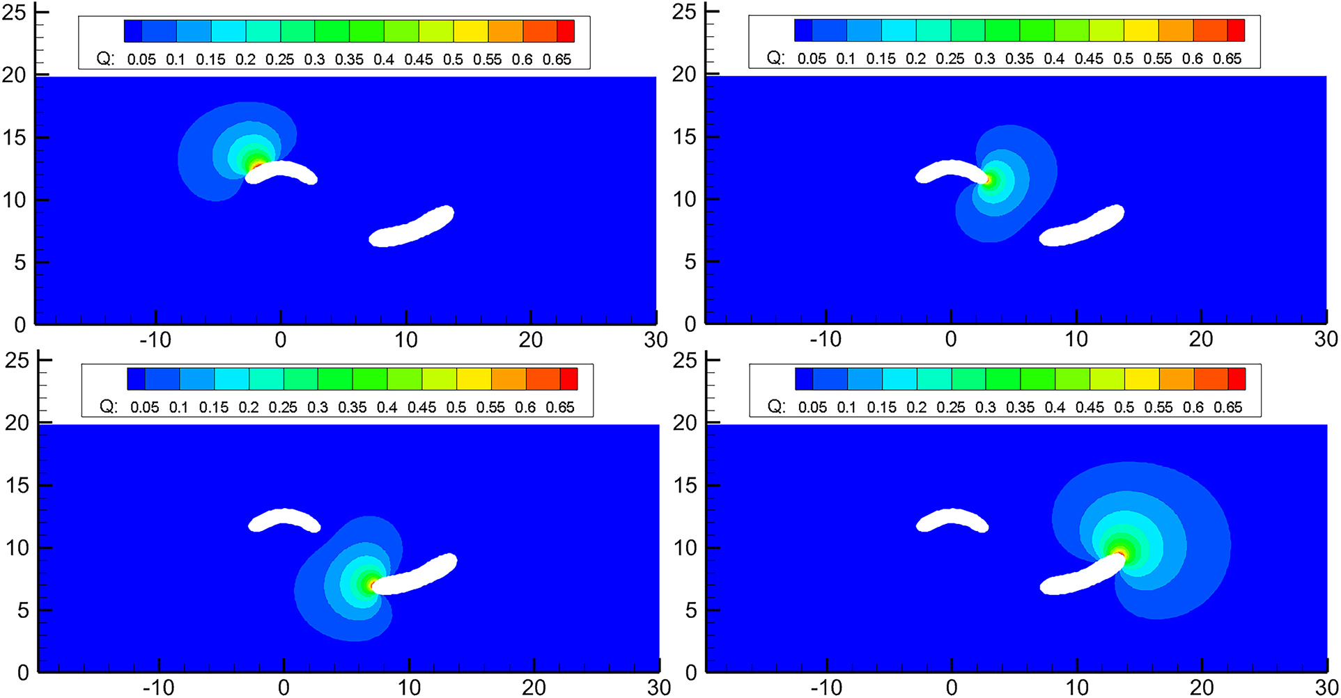
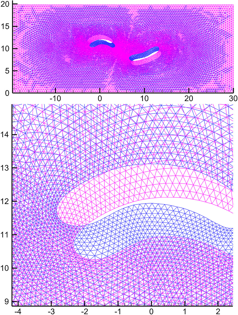
Figure 9.

A visual comparison between the initial (blue) and the deformed (red) grids (1^st test case).

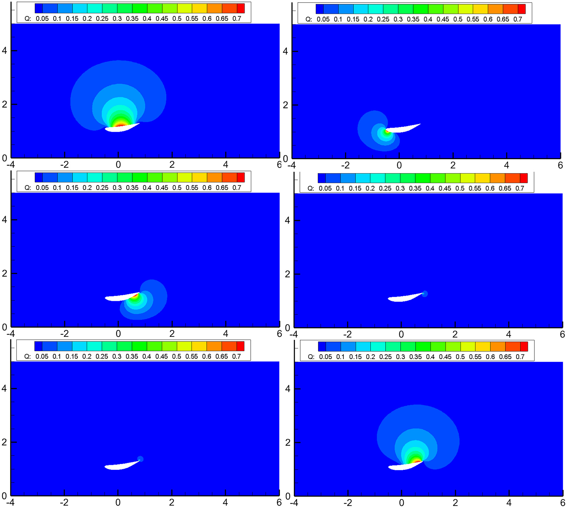
The second test case refers to an airfoil representing the diffuser of a Diffuser Augmented Wind Turbine (DAWT); it is formulated as a closed periodic B-spline curve of 2^nd degree with 14 (different) control points. In Figure 10 the solution to the Laplace’s equation is depicted, for only 6 of the basis functions (for control points: 1, 4, 7, 9, 12, and 14).

Figure 10.

The Harmonic Functions produced by the solution to the Laplace’s equation for 6 different B-spline basis functions (2^nd test case).

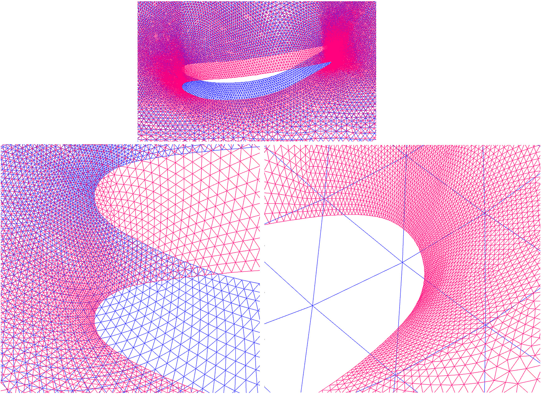
The applied movement to each one of the control points of the 2^nd test case, using the proposed methodology, results in the deformation of the entire unstructured grid, as depicted in Figure 11. It should be emphasized here that the initial grid is the one used for the consecutive solutions to the Laplace’s equation (while each deformed grid can be used for the solution to the flow equations, for the corresponding deformed airfoil geometry). A large deformation (equal for all control points) has been applied to demonstrate the ability of the methodology to handle such deformations.

Figure 11.

A visual comparison between the initial (blue) and the deformed (red) grids (2^nd test case).

Conclusions

The proposed methodology allows for the concurrent deformation of the curved boundaries and the corresponding computational mesh (structured or unstructured) in design optimization loops, without the need for a separate piecewise linear cage (and a separate computational grid for the Laplace’s equation). The deformation of the geometry boundaries is applied on the control points of the B-spline curves that describe the corresponding boundaries. Therefore, no reverse-engineering is required at the end of the optimization procedure to compute the parametric definition of the final geometry, which, eventually, is a known B-spline curve. The computation of the field of the harmonic functions requires significant computational resources, as this computation should be performed multiple times, equal to the number of the control points defining the B-spline boundaries (equal to the number of the corresponding basis functions, also used as boundary harmonic functions). However, this computation is performed only once, at the beginning of the deformation procedure (and does not include the non-deformed boundaries). The use of the described multigrid methodology, significantly accelerates the numerical solution, rendering the proposed methodology applicable to practical problems. Although the proposed methodology is very promising, the resulting quality of the deformed grid is not always perfect, especially when large deformations are applied. In some cases of large deformations negative volumes may result, very close to the deformed boundary. Therefore, further research is required to expand its potential for aerodynamic shape optimization.

Comparing (qualitatively) the proposed methodology with Free-form Deformation (FFD), the latter provides smoother mesh deformations, with better local control, as the lattice points (which control the deformation) extend inside the mesh region. On the other hand, at the end of the applied FFD deformation, the deformed geometry is not in a parametric form, and a reverse-engineering procedure is required to compute its parametric (B-spline or NURBS) form. In the proposed methodology the control points of the parametric B-spline curves that define the geometry boundaries control both the deformation of the geometry (boundaries) and the internal computational mesh. It should be mentioned here that the proposed methodology has been developed for periodic B-spline curves, which provide smooth basis functions.