
Introduction
Lean premixed combustion is widely utilized to minimize the emission of NOx by reducing the peak temperature within combustor, while simultaneously maintaining low levels of other pollutants (Correa, 1998; Lewis et al., 1999; Lefebvre and Ballal, 2010). However, the combustion process in lean premixed systems is highly sensitive to noise disturbances, which can lead to undesirable thermoacoustic instability (Poinsot, 2017). Thermoacoustic instability is a challenging problem in many combustion systems especially in gas turbine combustors, which can result in high-amplitude pressure oscillations leading to loud noise, reduced efficiency, and even risks of structural damage. This instability arises from the coupling between acoustic waves and heat release fluctuations within the system, causing pressure oscillations that can grow in amplitude and cause combustor instability. Passive control methods have been proposed as a promising means to mitigate thermoacoustic instability without requiring major modifications to combustion system hardware. One of such technologies is the Helmholtz resonator, which works by absorbing acoustic energy, thereby disrupting the coupling between acoustic waves and pressure fluctuations in the combustor.
When analyzing the performance of a Helmholtz resonator in suppressing thermoacoustic instability, an isolated description of damper behavior is insufficient and requires investigation of the coupled system between the resonator and combustor. In modern gas turbine combustors, the temperature of combustion products can reach over 2,000 K (Palies et al., 2011). This hot gas flowing through the combustor duct is known as grazing flow. To protect the HR structure from erosion by the hot gas, a cooling flow, referred to as bias flow, is often introduced from later several stages of the compressor through the HR back cavity, and then passing through the HR neck. The temperature of this bias flow is typically between 500–800 K, with low Mach numbers (generally not exceeding 0.3) (Royce, 2015). Usually, the cross-sectional area of the HR neck is much smaller than that of the combustor, leading to a much smaller ratio of the mean mass flow rate of bias flow to grazing flow, therefore the mean flow parameters of the grazing flow in the combustor is generally considered to change slightly up- and downstream the HR. For this reason, this temperature difference is often disregarded during modeling. However, it is important to note that the mass flux oscillation of bias flow may be of the same order of magnitude as that of the grazing flow near the resonant frequency. When the cooling bias flow mixes with the hot grazing flow within the combustor, temperature disturbances are produced, thereby generating significant entropy disturbances. This has been demonstrated to be crucial in predicting thermoacoustic oscillations, but only has received little attention (Li and Morgans, 2015; Yang and Morgans, 2017).
In certain circumstances, increasing suitably the bias flow is necessary to withstand the periodic invasion of hot grazing flow into the neck region (Bellucci et al., 2004; Ćosić et al., 2015; Bourquard and Noiray, 2019; Miniero et al., 2023). When the ratio between the mass flux of the bias flow and the grazing flow (also dependent on temperature and other parameters) reaches a non-negligible value, the difference up- and downstream the HR inside the combustor duct in mean flow parameters becomes significant and cannot be ignored. This will be studied in the present paper. This paper is organized in the following way. Firstly, a new acoustic analogy model is derived, considering the two temperature difference effects mentioned earlier. This model combines the principles of mass, momentum, and energy conservation with a linear Helmholtz resonator model. The numerical method and simulation strategy are then explained. Mesh independence tests and verification against experimental results were conducted. In the Results and Discussion section, a comparison is made between the derived theoretical model and three existing models, followed by further comparison with the numerical results. The impacts of the temperature difference are discussed. Finally, the Conclusion section summarizes the key findings of the study.
Theoretical model
Figure 1 illustrates a one-dimensional combustion chamber equipped with a Helmholtz resonator (HR) on its side wall. The schematic shows various parameters such as the HR neck length (l), the combustor duct cross-section area (Ac), the HR neck cross-section area
Governing equation
The conservation of mass, momentum and energy for this one-dimension combustion duct gives
whereIntegrating Equation. (1) from sections 1–2 yields the mean flow conservation equations. Then by giving mean flow parameters upstream the resonator,
Due to the dynamic mixing of cold and hot flows, the system will naturally generate entropy waves. Therefore, the density perturbation will include the effect of entropy perturbations
This is our one-dimensional acoustic wave governing equation.
In order to obtain the relation between the up- and downstream pressure disturbances, Equation (4) needs to be solved. Equation (4) degenerates to a homogeneous equation in the regions up- and downstream of the HR (in
where
By integrating once and twice of Equation (4) with respect to x across the source region, substituting the wave number Equation (6) and the expression for density disturbance
(7)
We note that integrating
where
Entropy model
In order to obtain the oscillating entropy
where
where
This expression demonstrates that the perturbation of entropy observed in the downstream section of the combustor depends on two factors, namely the variance in the mean stagnation enthalpy between the up-and downstream sections of the combustor as well as between the HR and downstream section of the combustor.
We have formulated a set of six equations, namely Equations (5), (7)–(9) and (11) with eight unknown perturbation parameters denoted by
(13)
To ensure that the system is well-defined, two boundary conditions must be imposed. Typically, the boundary condition for the inlet and outlet are fixed. If
We designate the solution of the acoustic analogy model considering mean flow discontinuity between the up- and downstream of the combustor as MAA. In the subsequent section, we will consider a test case with given boundary condition, and use the Linearized Navier-stokes (LNS) solver in COMSOL to validate the results.
Numerical simulation
To validate the theoretical model, numerical simulations were employed, considering non-steady, compressible, and non-isentropic characteristics to accurately depict information from a three-dimensional flow field. This can be achieved by creating a 3D model of a Helmholtz resonator and combustor duct using COMSOL Multiphysics. The mean flow field results obtained from Computational Fluid Dynamics (CFD) are utilized as the background mean flow. The type of CFD simulation employed in this study is the Reynolds-Averaged Navier-Stokes (RANS) model. These results are inserted into the acoustic mesh using a dedicated mapping module to solve the linearized Navier-Stokes (LNS) equations in the frequency domain. The LNS and CFD governing equations employed in this study are consistent with those described in references (Lu et al., 2019; Wu and Guan, 2021; Dastourani and Bahman-Jahromi, 2021; Zheng et al., 2023). The solution methodology employed in the present simulation adheres to a flowchart, depicted in Figure 2.
Table 1 presents the relevant fluid parameters utilized in both theoretical analysis and numerical simulations, as well as the geometric dimensions of the HR and combustor duct. Figure 3 shows a schematic view of the 3D model,
Table 1.
The geometries and flow conditions of the coupled HR-combustor model.
| Parameters | Values | Parameters | Values |
|---|---|---|---|
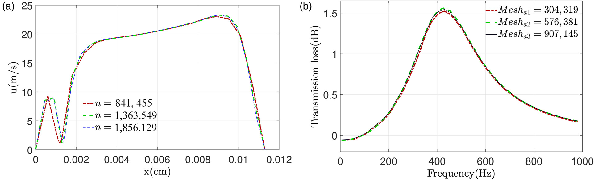
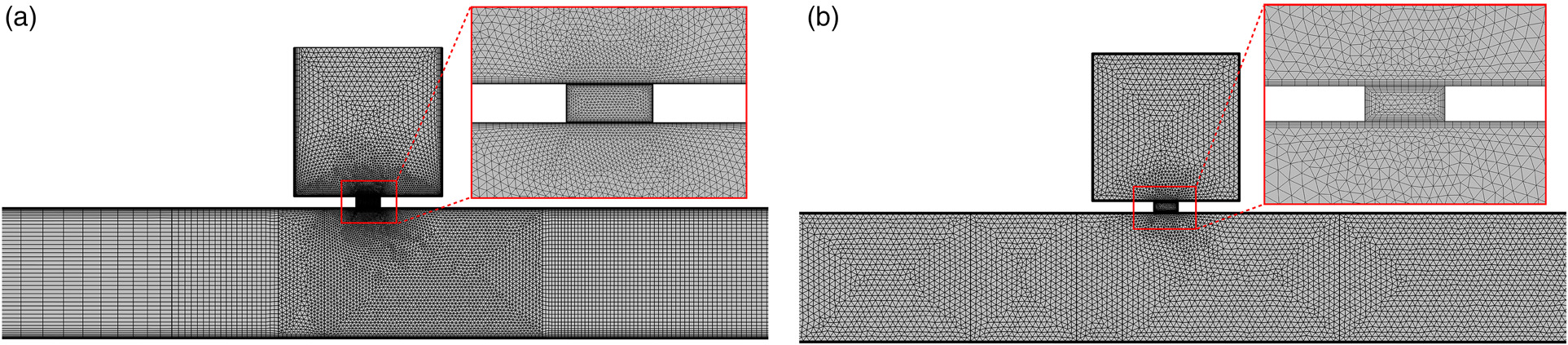
Mesh independence and verification test
In order to validate the accuracy of the modeling approach, the geometric parameters of the model were adjusted to match those used in the experimental (Selamet et al., 2011). The simulated transmission loss results were then compared with the experimental results, as illustrated in Figure 4. To validate the mesh independence of the results in the flow simulations, three meshes with different number of elements were employed, with a total of
Figure 4.
The comparison between the simulated transmission loss (TL) obtained from the model constructed using the current steps in COMSOL and the experimental results.
Results and discussion
We now consider a test case to study the effect of the temperature difference between the HR and combustor on the acoustics inside the combustor. In this case, we make the assumption that the upstream and downstream sections of the combustor duct are both infinitely long, i.e. non-reflecting boundary condition. An incident wave
Comparisons with previous models are performed to validate the present model in the isothermal case. Other different acoustic boundary conditions are also can consider to our model. Maintaining the bias flow temperature
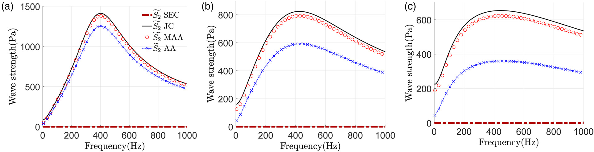
Figure 7.
Comparison of acoustic wave strength across various models and numerical results. (a) M ¯ n = 0.03 , m ¯ n / m ¯ 1 ≈ 5.1 % M ¯ n = 0.06 , m ¯ n / m ¯ 1 ≈ 10.2 % M ¯ n = 0.09 , m ¯ n / m ¯ 1 ≈ 15.3 %
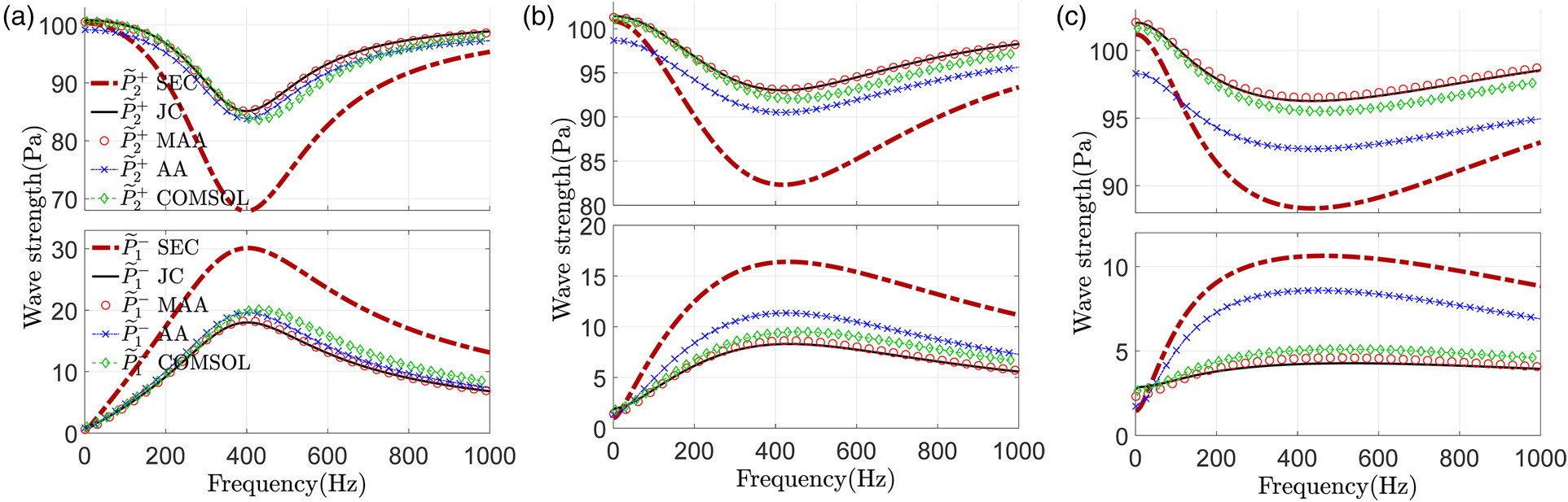
Figure 8.
Comparison of downstream duct transmission loss across various models and numerical results. (a) M ¯ n = 0.03 , m ¯ n / m ¯ 1 ≈ 5.1 % M ¯ n = 0.06 , m ¯ n / m ¯ 1 ≈ 10.2 % M ¯ n = 0.09 , m ¯ n / m ¯ 1 ≈ 15.3 %
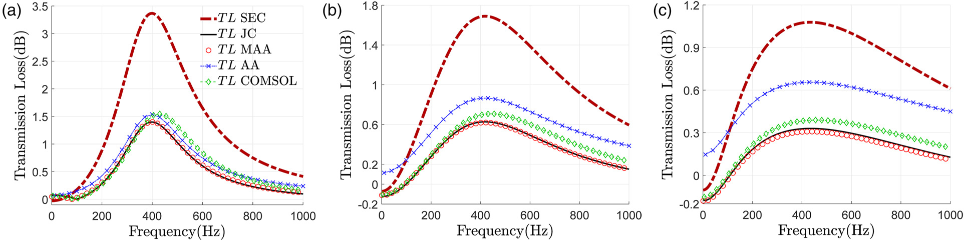
From Figures 7(a) and 8(a), it can be seen that when
The entropy wave strength can be defined as
Conclusion
In this paper, we extend our previous work on the acoustic analogy (AA) model (Gan and Yang, 2022) and propose a new model, MAA. The new model incorporates the effects of temperature difference between the upstream and downstream sides of the combustor in addition to the previously considered effects of temperature difference between the HR and the combustor. While the AA model provides a reasonable explanation for the acoustic effects in the combustor produced by the HR with cooling flow, the new MAA model is more general and includes the discontinuity effects of the mean flow parameters between the upstream and downstream regions of the combustion chamber. Comparing the theoretical and numerical results obtained from the COMSOL simulation, we find that when the ratio between the mean bias mass flux and the mean grazing mass flux does not exceed 10% in this study, the discontinuity effects of the mean flow parameters inside the combustor significantly will have negligible impact on acoustic and entropy wave strengths in the combustor. When this mass ratio is relatively large, ignoring this effect would result in overestimating the transmission loss in the combustor duct and underestimating the entropy waves strength generated downstream of the combustor. Moreover, the error increases with the increase of the bias mass flow rate. Therefore, in some cases where a large bias mass flow rate is required, it is necessary to consider both the temperature difference between the HR and the combustor and the temperature difference between the upstream and downstream regions of the combustor.
Nomenclature
Cp
heat capacity at constant pressure, J/(K · kg)
Rgas
the perfect gas constant
Revised Rayleigh conductivity
δ(x)
Dirac’s delta function
D
Dimeter, m
L
Length, m
A
Cross-sectional area, m2
V
The volume of the HR cavity, m3
m
Mass flux, kg/s
f
Momentum flux, kg·m/s2
e
Energy flux, kg·m2/s3
E
Stagnation enthalpy, J/kg
p
Pressure, Pa
s
Entropy, J/(K·kg)
S
Entropy oscillations strength, Pa
t
Time, s
x
Axial location, m
T
Temperature, K
u
Velocity, m/s
c
Speed of sound, m/s
ω
Angular frequency, rad/s
ρ
Density, kg/m3
k
The wavenumber, m−1
M
Mach number
γ
Heat capacity ratio