Introduction
The design of centrifugal compressors requires the use of computational methods in conjunction with experimental validation to provide accurate analysis with a quick turn-around between design iterations. The difficulty that arises when using computational methods is the simulation turnover time, which depends heavily on the grid used, boundary conditions applied and the turbulence model employed. Full-stage unsteady simulations are currently too costly and time consuming for the iterative design process. Steady-state models which use a mixing-plane method to model the interface between rotating and stationary domains are preferred due to the considerably reduced simulation time. However, the importance of turbulence model chosen still plays a significant role in achieving realistic predictions of the compressor performance.
Turbulence modelling attempts to model turbulent flow behaviour using a set of partial differential equations based on appropriate approximations of the exact Navier-Stokes equations 14. There are two types of Reynolds Averaged Navier Stokes (RANS) models that either (i) use the turbulent (or eddy) viscosity μt to calculate the Reynolds stresses or (ii) solve an equation for each of the Reynolds stresses. The eddy-viscosity models use the Boussinesq approximation, defined as the product of the eddy-viscosity and mean strain rate tensor to calculate the Reynolds stresses ().
The eddy-viscosity is calculated as a function of the modelled turbulent variables. This method assumes that the Reynolds stresses are isotropic, which is a valid assumption for simple flows. However, the Reynolds stresses are found to be anisotropic in complex swirling flows such as those present within a centrifugal compressor 14. Theoretically, the downside of eddy-viscosity models is that they are unable to properly account for streamline curvature, body forces and history effects on the individual components of the Reynolds stress tensor 04. Therefore, Reynolds stress models have potential advantages over their eddy-viscosity counterparts. However, with respect to centrifugal compressor flows, this is often not the case and strong similarities often exist between the two with respect to local flow field structure and performance parameter predictions. There are many different formulations of turbulence model, both of the eddy-viscosity and Reynolds stress type. The main factors that influences the selection process are the computational cost, grid requirements and ability to capture realistic flow physics.
Scope of paper
The present work is a comparative study of several different turbulence models used in the steady-state simulation of a centrifugal compressor stage with a vaned diffuser. The performance and flow field predictions are evaluated against experimental data and the results of each turbulence model are discussed. The primary objective of the present study is to propose a stable, numerically robust and accurate turbulence model suitable for application to flows within a centrifugal compressor over a broad range of operating conditions.
Centrifugal compressor stage
The centrifugal compressor stage used for the assessment of turbulence model predictions was the exemplar open test case, entitled “Radiver” 17. The compressor stage consists of an unshrouded impeller with 15 backswept blades and 23-vane wedge type diffuser. Numerical simulations were carried out at 80% design speed due to the large amount of experimental data available for comparison to CFD predictions. Details of the impeller and diffuser geometry are contained in Table 1.
Table 1.
Compressor details for 4% radial gap at 80% speed.
Numerical details
Solver
Simulations were carried out using the commercial CFD code ANSYS CFX 16.2. A high resolution advection scheme was used to solve the discretised conservation equations and mass flow was evaluated using the high resolution velocity-pressure algorithm of Rhie and Chow based on the numerical set-up of 05. Second order turbulence numerics was selected and a turbulence intensity of 5% assumed at the inlet of the computational domain according to recommendations 02 and a similar case 10. Conservation of energy was evaluated using the total energy equation with the viscous work term included to capture any heat generation due to viscosity.
Modelling approach
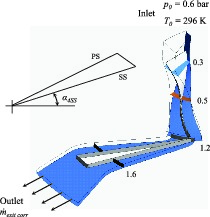
Numerical simulations were performed using a steady-state, single-passage model with periodic boundary conditions, as shown in Figure 1. Structured hexahedral grids for the impeller and vaned diffuser passages were generated using the dedicated ANSYS meshing tool TurboGrid.
A mixing-plane (or “stage”) interface was used at the interface of the rotating impeller and stationary diffuser domains. The stage interface performs a circumferential averaging of the fluxes at the exit plane of the rotating domain to construct spanwise profiles of the conserved variables at the inlet of the stationary domain. Stage averaging between the blade passages accounts for time averaging effects, thus the results do not depend on the relative position between the two components.
Since the collector at the outlet of the diffuser is not included in this analysis, the computational domain is restricted between an inlet plane 50 mm upstream of the impeller leading edge (the measurement plane 1) to shortly downstream of the diffuser exit (8M); according to the notation in 17. Thus, the performance is evaluated between the planes 1 and 8M. This is also similar to the computational setup used by 10.
Boundary conditions
The inlet conditions were specified as a total pressure of 0.6 bar and a total temperature of 296 K (23°C) based on recommendations by the authors of the test case. The fluid is defined as Air Ideal Gas and the no-slip boundary condition was defined at all solid wall surfaces. The specific heat capacity at constant pressure Cp and ratio of specific heats γ are 1005 J/kg·K and 1.4, respectively.
It is known that CFD solvers run into difficulty at/near the stall/surge and choked flow conditions depending on the outlet boundary condition specified. Typically, a static pressure boundary condition is placed at the outlet near choke conditions and a mass flow rate boundary condition near stall/surge 05, 09. In this analysis, the exit corrected mass flow rate ṁexit corr has been used. It is a function of the stage mass flow rate, and mass averaged total temperature and pressure at the outlet plane, 8M 02. This makes it more stable compared to a static pressure or regular mass flow rate condition. Finally, the location of the impeller-diffuser interface is mid-way along the radial gap of 4% r2; this corresponds to a radius of 137.7 mm.
Three operating points were simulated along the 80% speedline (P1 [near surge], M [mid-speedline] and S1 [near choke]) to determine how each turbulence model performs under different operating conditions.
Grid convergence study
A grid convergence analysis was carried out to ensure that the solution was grid independent and the discretisation error low. Three grids, namely coarse, medium and fine were simulated at the operating points P1, M and S1 using the SST turbulence model. This model was chosen for its numerical stability over a range of operating conditions 05. Also, the converged mesh can be applied to the SST-CC and RSM-ω models due to their similar grid requirements. A target y+ value of 0.7 was used to ensure the change in turbulence model did not have a profound effect and to have a good boundary layer resolution. The number of elements for each grid from coarse to fine was 0.5 million (0.5M), 1M and 2M. Convergence was deemed to be achieved whenever the RMS residuals were less than 1E-04, and the global imbalances of mass, momentum and energy are less than 0.1%. The percentage change in several overall parameters for operating point P1 are shown in Table 2. It is clear that the discrepancy for the first grid refinement (coarse to medium) is much more significant than the second refinement (medium to fine).
Table 2.
Absolute percentage discrepancy between grid refinements at the operating point P1.
| η01,08M | П01,08M | η01,8M | П01,8M | TR01,08M | |
|---|---|---|---|---|---|
| C-M | 1.46 | 1.07 | 3.18 | 2.48 | 0.05 |
| M-F | 0.41 | 0.50 | 0.57 | 0.63 | 0.04 |
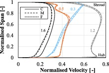
Another method used for analysing the simulations for grid independence was by comparing circumferentially mass averaged, spanwise velocity profiles at a number of streamwise locations through the compressor stage. The streamwise locations of the turbosurfaces used to compute the velocity profiles can be seen in Figure 1. The velocity profiles are non-dimensionalised by the blade tip speed U2 (≈ 403 m/s). In the rotating and stationary frames of reference, the relative and absolute velocities are used respectively.
The normalised velocity is shown in Figure 2 for operating point P1, where the line colours correspond to the streamwise planes defined in Figure 1. The coarse grid shows a larger difference near diffuser channel exit compared to the medium and fine grids. This is due to an increased level of blockage predicted within the diffuser channel compared to the other two grids, where specifically, the coarse grid predicts 25% and the medium and fine grids predict approximately 15% channel blockage. Based on the results of the grid convergence analysis, the medium grid is chosen as a trade-off between accuracy and computational solve time. Please refer to the Appendix for grid convergence plots and absolute percentage discrepancy between grid refinements at operating points M and S1.
Selected turbulence models
Eddy-viscosity models
The first eddy-viscosity model considered in this study is the SST model which is a combination of the k-ɛ and k-ω turbulence models where the former model is used for the free stream flow and the latter is used for modelling near the wall. Mathematical blending functions are employed to switch between models without user interaction 08. The SST has been applied frequently to model centrifugal compressor flows in recent times as it provides good predictions of the flow field and compressor performance over a broad range of operating conditions. However, it is not perfect as it often over predicts the stage total pressure rise 11.
Since eddy-viscosity models are insensitive to streamline curvature and system rotation, a number of modifications have been suggested to sensitise them with little solver implementation and effort. 12 proposed a modification to the production term Pk in order to sensitise eddy-viscosity models to these effects. In regions of enhanced turbulence production such as a strong concave surface, the multiplication factor takes on a maximum value of 1.25 whereas in regions of no turbulence production such as a strong convex surface, a value of 0 is used.
The other eddy-viscosity model investigated is the SA turbulence model. This one-equation turbulence model uses a transport equation for the modified turbulent kinematic viscosity. The major advantage of this model is that it uses only one transport equation, as opposed to two of the SST model, making it efficient with respect to computational time.
Reynolds stress models
The RSM-SSG turbulence model solves for each Reynolds stress using the turbulence dissipation rate ɛ, a quadratic pressure-strain correlation and employs scalable wall functions in 03. 07 states that the pressure-strain correlation “represents the redistribution of energy between different components of the turbulence”. The additional terms proposed by Speziale, Sarkar and Gatski (SSG) are found to provide a more accurate representation of turbulent flows 14.
The RSM-ω model solves for each of the Reynolds stresses using the turbulence frequency ω as the transport variable. An advantage of this model over the RSM-SSG is that it does not use the turbulence dissipation rate which is found to be problematic in regions of large separation. Furthermore, automatic wall functions are employed to provide accurate resolution into the boundary layer based on the grid used. Whilst the current literature does not show much application to turbomachinery flows, 06 found that the results obtained were similar to the SST model when investigating turbulent flow and heat transfer in a square-section duct.
Results and discussion
The following sections present the results obtained by each turbulence model. Where possible, predictions are compared to experimental data. One-dimensional data is available for all operating points considered, e.g., pressure and temperature, whereas local experimental contour plots are available only for the operating points P1 and M.
Global speedlines
Firstly, the global performance predictions of the compressor stage are presented in the form of speedlines. Speedlines are shown in Figure 3 for a number of different performance measures of the compressor. The data is normalised using the experimental values at the operating point M. Each model predicts the performance of the compressor in good agreement with the experiment in most cases, where the differences from the experiment are generally quite small (less than 2% in most cases). The pressure ratio is predicted in good agreement with the experiment by each turbulence model. However, the total-to-total efficiency suffers because of the discrepancy in total temperature at the outlet, particularly near the choke condition. The absolute percentage discrepancy between experimental and numerical results for the operating point P1 is listed in Table 3. Please refer to the Appendix for absolute percentage discrepancy between experimental and numerical results at operating points M and S1.
Table 3.
Absolute percentage discrepancy between the experimental and numerical results at P1.
| SST | SST-CC | SA | RSM-SSG | RSM-ω | |
|---|---|---|---|---|---|
| П01,08M | 0.69 | 0.28 | 0.64 | 0.68 | 0.77 |
| η01,08M | 1.83 | 1.61 | 0.77 | 1.77 | 2.18 |
| η01,8M | 0.83 | 1.05 | 3.43 | 1.48 | 1.33 |
| TR01,08M | 0.27 | 0.35 | 0.01 | 0.27 | 0.35 |
Figure 3.
Global performance parameters (a) total-to-total pressure ratio, (b) total-to-total temperature ratio, and (c) total-to-static efficiency.
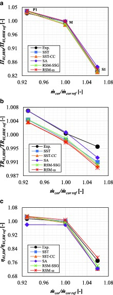
SA predicts the total-to-total pressure and temperature ratio in good agreement with the experiment at the operating point P1 and it predicts the total-to-total efficiency most accurately of all the models considered. However, it is the least accurate in terms of total-to-static efficiency. The reason for this is addressed in detail later. The curvature correction applied to the SST model reduces the discrepancy in terms of total-to-total pressure ratio. This is in agreement with 11 and 01. However, the main drawback of the correction is in the form of a slightly reduced work input (due to the lower total temperature at the outlet relative to the original SST model; Figure 3. The RSM-SSG is slightly better than the RSM-ω however, the differences between the models are not significant.
The operating point M is predicted with better accuracy than P1, where differences are well below 1% in most cases. An interesting feature at this operating point is the shifting of the RSM-SSG and SST-CC below the experiment with respect to total-to-static efficiency; Figure 3. Inspection of the static pressure at diffuser exit highlights that both models under predict the static pressure by 1.04% (RSM-SSG) and 1.50% (SST-CC and SA). This, in combination with a reduced work input predicted, is the main contributor towards a lower efficiency prediction.
Near the choke condition (S1), the performance is not relatively well predicted by many of the models. The reason is attributed to the flow becoming highly separated within the diffuser. An interesting feature at this point is that the RSM-ω is the only one to over predict the total-to-static efficiency whereas the other models are found to under predict this parameter. This is attributed to the small discrepancy in static pressure at diffuser outlet (0.15%) where the others predicted well above 3%. Conclusively, all five models provide the overall performance parameters within an acceptable range of accuracy for the present test cases.
Local measurement plane comparison
Impeller exit: Measurement plane 2M’
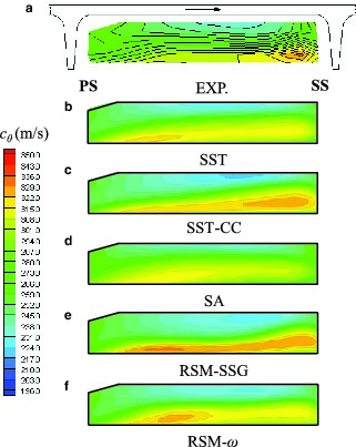
For the near surge operating point P1, absolute (c), meridional (cr), circumferential (cθ), and relative (w) velocity distributions were compared at the impeller exit plane, 2M’. The circumferential velocity contours among those are shown in Figure 4. In general, the SST-CC turbulence model showed the best prediction of the local flow structures of the secondary vortical flows in the impeller, whilst the SA showed the least accurate flow field prediction. There were close similarities between the SST-CC and RSM-SSG models although the RSM-SSG magnified the intensity of localised features near the shroud significantly. Regarding the SA turbulence model, it is unique in that it did not predict the highly localised secondary flows like the others i.e., the flow field was more homogenous indicating less loss by the secondary flows.
Figure 4.
Circumferential velocity contours for different turbulence models at the impeller exit (plane 2M’) and the operating point P1.
In order to understand the development of the secondary vortical flows within the impeller passage and compare them between the SST-CC and SA model predictions, the vorticity contours at two different cross-sectional planes are plotted in Figure 5 and Figure 6. The streamwise locations of these planes are according to the notation shown in Figure 1. Near the inducer inlet, the inceptions of the secondary flows, such as tip leakage flow near the shroud and the passage vortices (the wake of low pressure near the shroud and the jet of high pressure in the main passage) are observed. The flow fields of two models are almost the same (not shown here). Only the magnitude of vorticity near the walls predicted by the SST-CC is marginally higher than that of the SA. However, this discrepancy accumulates along the impeller passage.
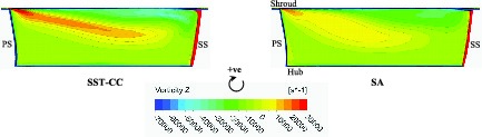
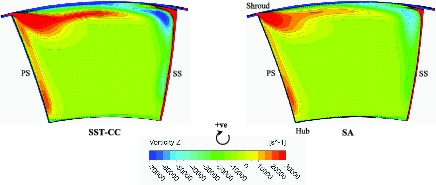
Notable differences between SST-CC and SA predictions begin to appear in the axial-to-radial elbow of the impeller channel. Figure 5 depicts the vorticity contours at the plane of the streamwise location of 0.45, where the blade surface vortices are generated by the meridional curvature 13. As the radius of the meridional curvature is smaller near the shroud, larger vortices have been seen near the shroud; the gradient of the relative velocity is stronger near the suction side boundary layer. As a result, the stronger vorticity can be seen near the suction side shroud region. The vortices predicted by the SST-CC model are stronger than those by the SA model as shown in Figure 5.
The blade surface vortices dissipate gradually towards the impeller exit. In this context, the strength of the vortices near the blade surfaces decreases from the plane (at 0.45) in Figure 5 to the downstream plane (at 0.65) in Figure 6. As can be seen in Figure 6, the low wake vortex of the passage vortices near the shroud is enlarged toward the impeller outlet, whilst the high jet vortex of the passage vortices is reduced along this direction. The secondary flow near the shroud wall from suction to pressure side, (opposite to the shroud passage vortex, as well as the tip leakage vortex near the shroud suction side corner) are clear and significant in the case of the SST-CC model prediction. However, the SA model prediction shows a relatively larger drop of the vorticity strength in the downstream plane (Figure 6), and the secondary vortices are smeared. The SA model is the only model not to predict the localised region of strong negative vorticity near the shroud suction side corner; a feature reported by 16.
The secondary vortical flows are closely related to the loss generated in the passage. The magnitude of loss predicted by the SA model is the lowest due to under prediction of the secondary flow effects as formerly described; this finding is in agreement with 15. The SA model is the only one to consistently over predict the pressure ratio and efficiency of the impeller at all three operating points and has the largest discrepancy of the stage total-to-static efficiency from the experimental results. In the present case, the curvature correction function applied to the production term of the SST model aids in the prediction of a more accurate cθ distribution; Figure 4.
It is well known that the circumferential averaging performed at the mixing-plane interface between the impeller and diffuser domains can introduce significant errors downstream. The study of the Radiver compressor by 10 highlighted a large discrepancy between experimental and numerical (circumferential and spanwise) incidence angle at the measurement plane 4M (just upstream of the diffuser leading edge). This discrepancy across the mixing-plane led to an incorrect prediction of the Mach number distribution downstream of the diffuser channel exit (measurement plane 7M) due to incorrect flow separation within the diffuser section.
The spanwise eddy-viscosity μt distribution just upstream and just downstream of the mixing-plane interface is shown in Figure 7. The profiles are constructed by circumferentially averaging the eddy-viscosity along the spanwise direction from hub to shroud. The SA model predicts the largest level of turbulent eddies with the maximum in the central region, whereas the other models show one-sided distributions and larger eddy-viscosity near the shroud. This is attributed to the prediction of the secondary vortical flows in the shroud side as shown in Figure 6. Furthermore, this results in the discrepancy in the flow structures in the diffuser channel as discussed in the following sections.
Diffuser exit: Measurement plane 7M
The experiments by 17 found that the size of the radial gap influenced which side the maximum total pressure was biased towards in the diffuser channel at a fixed operating point. For example, at the operating point P1 for the 14% r2 gap it was biased towards the suction side and moved towards the pressure side with decreasing radial gap. For the 4% r2 gap, the total pressure was expected to be biased towards the pressure side and centre of the channel respectively for operating points P1 and M respectively. Inspection of each turbulence model highlighted that the best model to predict the similar flow structure at this plane for the operating point P1 was the RSM-ω, although the wake was predicted larger near the pressure side; Figure 8. At this near surge operating point, the separated flow and wake are the key flow features and discussed further in the subsequent section. The most unphysical model was the SA which showed a very highly loaded suction side compared to others which are more central; Figure 8. Although most models predicted the overall performance parameters in good agreement with the experiment, this does not imply that the flow features are too. In cases where the local flow structures must be accurately captured, the SA model does not appear to be appropriate.
Blockage and loss
Blockage has an adverse effect on the flow due to thick boundary layers altering the geometry of the flow passage. Unfortunately, there is no experimental data available to calculate the level of blockage (B2) at 2M’. However, it is interesting to inspect how blockage predictions at the impeller trailing edge varies between models at the operating point P1. In addition, the static pressure rise cp and stagnation pressure loss Yp through the diffuser are presented in Table 4, for which there is experimental data available for comparison. Both coefficients are evaluated between planes 2M and 7M i.e., just upstream of the diffuser leading edge and just downstream of the diffuser channel exit.
Table 4.
Comparison of blockage and diffuser parameters at P1.
| SST | SST-CC | SA | RSM-SSG | RSM-ω | Exp | |
|---|---|---|---|---|---|---|
| cp | 0.75 | 0.76 | 0.62 | 0.77 | 0.76 | 0.75 |
| Yp | 0.14 | 0.14 | 0.19 | 0.15 | 0.14 | 0.17 |
| B2 [%] | 16.32 | 17.66 | 14.84 | 14.34 | 13.58 | - |
Most models predict the static pressure rise across the diffuser in good agreement with the experiment, particularly the SST and RSM-ω, whereas the stagnation pressure loss is slightly lower for all models but the SA model. The values of cp and Yp reported by the SA model are not surprising since it has predicted the lowest total-to-static efficiency. The reasons for this are detailed below.
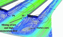
The diffuser vane wake produces a large level of loss within the diffuser domain due to recirculating flow that mixes with the flow exiting the diffuser channel near the suction side and also re-enters the separated pressure side flow. Figure 9 highlights this for the SA model which is found to predict the largest level of separation and lowest static pressure rise at the operating point P1. A closer inspection using three-dimensional velocity streamlines suggests that a clockwise rotating vortex (as viewed from above) and the pressure difference between the outlet and further upstream, is the mechanism behind the wake flow mixing with the separated flow on the pressure side of the vane. Although back flow downstream of the diffuser near the collector (which was not modelled) has been reported in the experimental test case, the magnitude of this has not been quantified. Therefore, in the case of the SA model, the location of the outlet plane at 8M may magnify the effect of the vortex behind the diffuser vane compared to the other models.
Since the SST model predicts the static pressure rise and the stagnation pressure loss coefficient in good agreement with the experiment, this model was used as a basis for comparison to the SA model with respect to entropy within the diffuser channel; Figure 10. Furthermore, at this off-design operating point (P1), the SST predicts the static pressure and total-to-static efficiency best out of all models (-0.03% and 0.833% respectively) implying that this model reflects the experiment realistically with respect to one-dimensional values.
Figure 10.
Static entropy contours at several streamwise locations within the diffuser domain (a) SA model, (b) SST model.
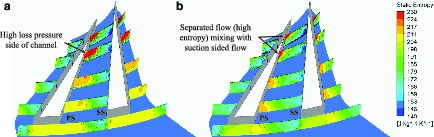
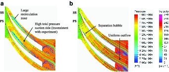
Within the diffuser channel, the SA model predicts a high level of entropy generation beginning shortly downstream of the diffuser throat, which spreads towards the centre of the channel, mixing with the low entropy flow near the suction side, and subsequently introduces further losses. On the other hand, the SST model predicts a similar level of entropy generation downstream of the diffuser throat on the pressure side in a relatively small region, but does not tend to spread further downstream. This relatively short passage of high entropy predicted by the SST model is due to a small separation bubble near the shroud, whereas the SA model shows large flow separation. Figure 11 shows a static pressure contour plot at 95% span in the diffuser domain with streamlines superimposed. The location of the separation bubble at the pressure side of the diffuser channel is visible and it can also be seen that the static pressure in the diffuser exit region is lower for the SA. The RSM-ω model shows a similar flow in the diffuser to that of the SST model, except the small separation is a bit further downstream than that of the SST model.
Computational time required
Simulations were carried out using an Intel Xeon 8 core processor. The “Platform MPI Local Parallel” function available within CFX was used to reduce computational time by utilising the total number of cores available.
The required wall clock time as well as the number of iterations to reach convergence are presented in Table 5. Clearly, the SST model is the most efficient with respect to time but also in terms of stability and robustness across the three operating points considered. Interestingly, the curvature correction has had a detrimental effect on the time required to reach convergence, contrary to 10 who noted that the convergence rate and total CPU time was similar at all operating points between the two models. However, in this study a denser grid (1.35 times more elements) has been used and the likely difference between the two is the solver struggling to resolve local flow instabilities. The most difficult model to reach convergence at each operating point was the RSM-ω in which the simulation had to be heavily relaxed to reach convergence. As expected, away from the stall/surge condition, the SA is the most efficient with respect to wall clock time and number of iterations to convergence.
Conclusions and recommendations
A number of turbulence models (SA, SST, SST-CC, RSM-SSG and RSM-ω) have been assessed and compared to experimental data of the centrifugal compressor, Radiver. For the compressor global performance parameters, each of the models assessed yielded good agreement with experimental results, where the discrepancy is well below 2% in most cases. The SST model provides accurate results over the entire speedline of the present test cases whilst keeping the solution time low. The increased accuracy in the prediction of pressure ratio and efficiency by the SST-CC model near surge compared to the original SST comes at the expense of a longer computing time (double in some cases). All Reynolds stress models were found to have a longer running time.
In terms of local flow field predictions, at the near surge operating condition P1, the SST-CC provides the most accurate results for all four velocities considered at measurement plane 2M’ (impeller exit, upstream of the interface), where comparable results are reported by the other eddy-viscosity models. On the other hand, the Reynolds stress models typically over predict the velocity near the pressure side of the blade due to the high intensity tip leakage vortex predicted. The SA shows the least accuracy at this plane. At measurement plane 7M (diffuser exit, downstream of the interface), the RSM-ω predicts the flow structure of wake and separation for the operating point P1 in fair agreement with the experiment, where the total pressure is slightly more central and the pressure side wake is larger. On the other hand, the SA fails to predict the proper flow structures with high levels of separation beginning just downstream of the diffuser throat. Consequently, this model predicts the static pressure and total-to-static efficiency least accurately. The SA predicts the work input by the impeller in excellent agreement with the experiment near surge and the mid-point of the speedline and is also the least computationally expensive near the mid-point and choke condition. However, one-dimensional averaging of the variables to calculate performance parameters conceals the local flow features and does not imply good resolution thereof.
In conclusion, even though the SST-CC and RSM-ω showed better performance in complex flow prediction near surge, the SST model is reasonably stable, robust and time efficient to predict the basic local flow physics and provides a good prediction of all performance parameters. The SA model is quick and provides comparable overall parameters. However, it shows some limits, such as the consistent under prediction of the static pressure at the outlet and inaccurate prediction of detailed flow structures. Therefore, the SA model is not recommended for detailed or advanced design stage prediction.