Description of the large eddy simulations software for flame transfer function calculations

Recently, LES has been used to perform simulations of self-excited thermoacoustic instabilities 25, 35 and to perform forced simulations to determinate the FTF 25, 36. In this article, results of LES, particularly FTF, described by 26 are used. To improve reading of the article, the description of LES is provided. The reactive multi-species Navier-Stokes equations on unstructured grids are solved using a fully compressible explicit code AVBP 28. The viscous stress tensor, the heat diffusion vector and the species molecular transport use gradient approaches. The fluid viscosity follows the Sutherland law and the species diffusion coefficients are obtained using a constant specie Schmidt number and diffusion velocity corrections for mass conservation 09. A high-order finite element scheme is used for both time and space discretisation. The turbulent stress term is modelled by the classical Smagorinsky model 34. A chemical mechanism with six species (CH₄, O₂, CO₂, CO, H₂O and N₂) and three reactions 27

is used to model methane/air combustion. The dynamic thickened flame model 05 is adopted to describe the iteration between turbulence and chemistry.

Usage of low-Mach number or “incompressible LES” 08 can give the advantage of shorter calculation times. Compressible LES are performed in this study, because in compressible LES, fewer approximations are made, thus they give more precise results.

Time-lag-distributed model for flame transfer function

In general, heat release rate Q oscillations of technically premixed swirl-stabilised flames depend on perturbations of velocity u and equivalence ratio φ 11

First, let us consider the response of the flame to upstream velocity perturbations. Once longitudinal acoustic wave reaches a burner swirler, it is divided into two components: oscillations of axial velocity and oscillations of tangential velocity. 17 have shown that the response of perfectly premixed swirl-stabilised flame to velocity fluctuations depends on both oscillations of two components of velocity — axial and tangential — and have proposed the time-lag-distributed model of the flame response to upstream velocity fluctuations.

where τ_i is the time delay of the corresponding mechanism, σ_i is the standard deviation of the corresponding time delay. The response of the flame to the axial perturbations of the velocity is modelled with the parameters τ₁ and σ₁. The parameters τ₂, σ₂, τ₃ and σ₃ model the response of the heat release to the tangential perturbations of the velocity produced by a swirler.

The physical meaning of the parameters τ_i and σ_i is understood if we switch from the frequency-domain representation of the FTF to its time-domain representation, i.e., to the unit impulse response (UIR). The UIR in this study is the response of the normalised heat release to the normalised velocity perturbation of unit amplitude. The analytical form of the UIR corresponding to the FTF of (4) is

Thus, (5) models the response of the heat release to acoustic oscillations with three Gaussians with mean values τ_i and standard deviations σ_i. The first Gaussian in (5) described with pair of parameters τ₁, σ₁ models the time that fluid particles spend to travel from the zones where the flame is anchored to different points at the flame. Parameters τ₂, σ₂, τ₃ and σ₃ model the time that a fluid particle spends to travel from the swirler to the flame.

01 have shown that the equivalence ratio fluctuations influence the heat release through three mechanisms: change of the heat of reaction, change of the flame speed and change of the flame surface area. It can be seen from Figure 4 of 12 that the response of the turbulent flame to equivalence ratio fluctuations could be modelled similarly to (4) and (5).

where parameters τ₄, σ₄, τ₅ and σ₅ together model the flame response to change of the heat of reaction and change of the flame speed, and parameters τ₆ and σ₆ model the flame response to area changes. Parameters τ₄, σ₄, τ₅, σ₅, τ₆ and σ₆ model the time that fluid particle spends to travel from the point of the fuel injection to different points at the flame.

Many gas turbines burners, including the burner under consideration, are designed in such way that the pressure drop of the gas through the burner is around one order of magnitude higher than the pressure drop of the air. In this case, the acoustic perturbations in the gas turbine combustion chamber excite oscillations of the air mass flow through the burner; meanwhile, the gas mass flow remains almost unperturbed. This allows to make an assumption that the equivalence ratio φ perturbations depend only on the air flow velocity u fluctuations in the burner 29

For such burners, it is possible to write a model for the total FTF.

where the fluctuations of the flame heat release rate Q′ depend only on the velocity fluctuations u′r at a reference position r upstream of the flame

At this point, the model for the FTF consists of 12 parameters and it could be cumbersome to determine all of them. However, for burners that have the fuel injection at the swirler blades, the values of the characteristic time delays modelled by parameters τ₄ and τ₆ are close to the values of the characteristic time delays modelled by parameters τ₂ and τ₃, respectively, and they cancel the resulting effect of each other. Thus, the model in (10) can be further simplified using only four parameters 29, 06.

Two Gaussians described by (11) and (12) model in a simplified way the change of the heat release due to perturbations of the velocity themselves and due to perturbations of equivalence ratio, respectively. They have the same relative amplitudes because increasing the velocity of the flow by certain relative value or decreasing equivalence ratio by the same relative value would increase heat release by the same relative value.

The FTF model described by (11) is used further in this study.

Wave-based approach for thermoacoustic simulations

When the length of the setup under consideration is much larger than its dimensions in the other directions, it is possible to perform a one-dimensional low-order acoustic analysis 02, 30, 03, 15.

The test rig is considered as a set of sections with constant cross-sectional area. Pressure, velocity, temperature and density are decomposed into the sum of their mean component (denoted by ¯) and their fluctuating component (denoted by ′). Mean values of pressure, velocity, temperature, density and thermophysical properties are assumed to be constant along each section and are changing only from section to section.

Perturbations of pressure p, velocity u and density ρ in each section could be represented in terms of downstream and upstream propagating acoustic waves (characteristics) (see Figure 1):

Figure 1.

Scheme of waves propagation in a section of a low-order acoustic model.

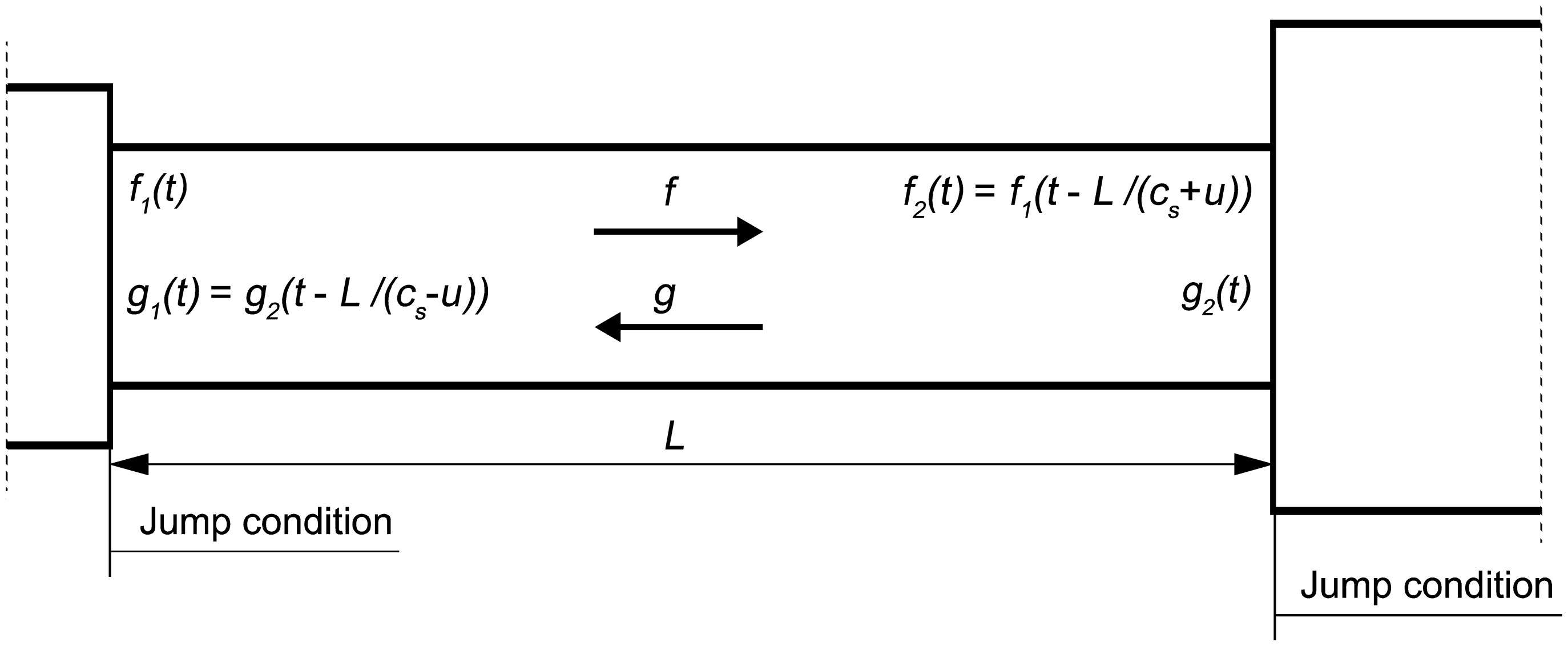
where f and g are the downstream and upstream travelling components (Riemann invariants) of acoustic waves, respectively, and c¯s is the mean speed of sound in the section.

In order to connect oscillating variables in different sections (see Figure 2), we need to know the jump conditions. To compute the jump conditions between sections separated by a compact acoustic element, such as sharp cross-sectional area change and a compact swirler, the system of linearised equations of conservation of mass and Bernoulli 07, 15 written in terms of f and g is solved.

Figure 2.

Scheme of waves propagation between sections of a low-order acoustic model.

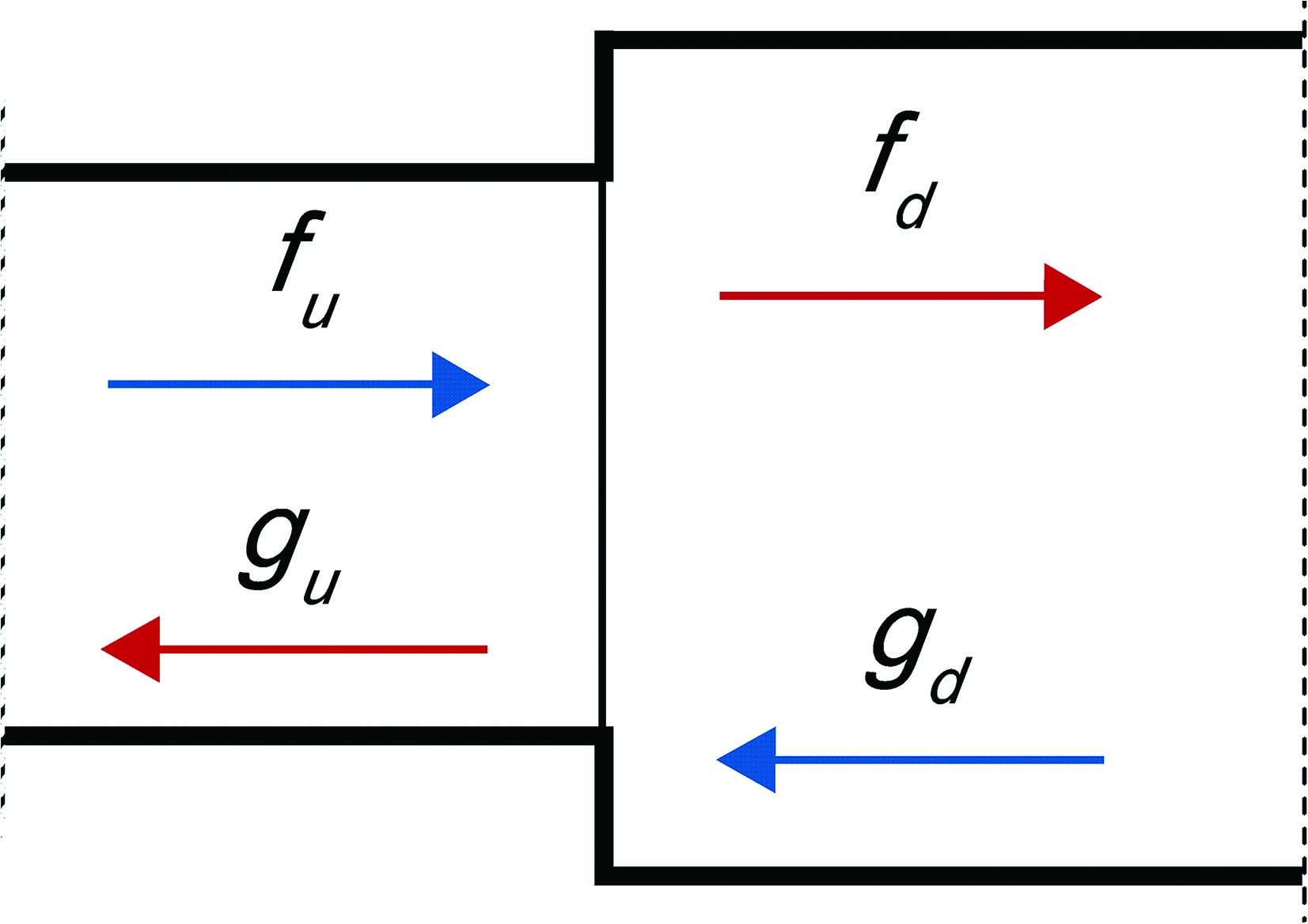
where subscripts u and d denote the upstream and downstream sections, respectively. Matrices F and K take into account acoustic losses between sections; their coefficients can be found in Appendix A..

To calculate the jump conditions at the flame, the system of linearised equations of conservation of momentum and energy (product of mass conservation equation and Bernoulli equation) written in terms of f and g is solved 07, 15.

where coefficients of matrices J and H can be found in Appendix A.. (16) and (17) are directly used in the network model time-domain simulations.

At the beginning of the first section and at the end of the last section, f and g waves are related by the reflection coefficients R_inlet and R_outlet, respectively.

There are four main sources of acoustic losses: at cross-sectional area changes, at partially reflective boundaries, at acoustic boundary layers and due to viscose dissipation. In this study, only the first two mechanisms of acoustic losses are taken into account.

Since the network model is implemented in Simulink, it is possible to design and test both active and passive dampers of thermally driven acoustic oscillations in future work.

Description of the experimental setup

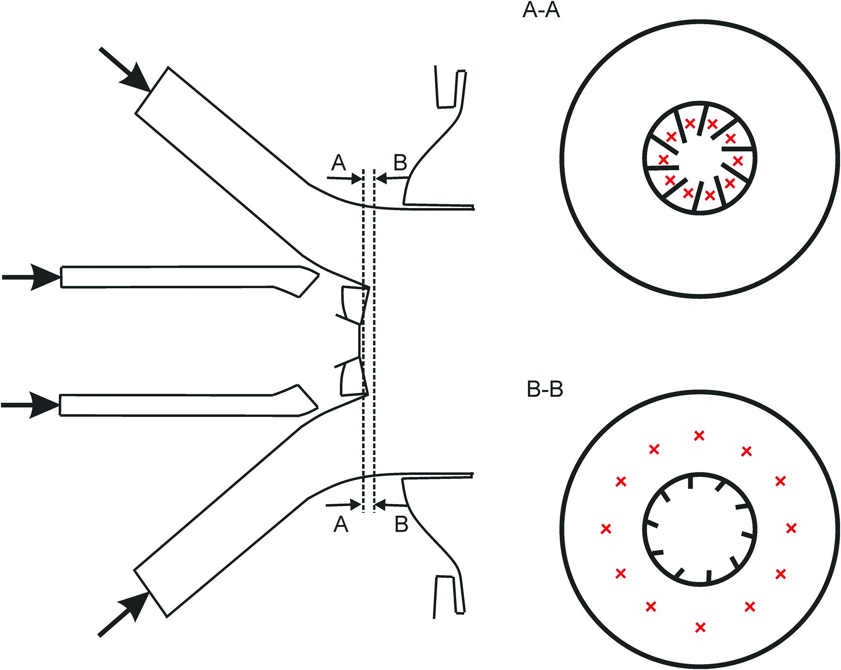
The atmospheric test rig is characterised by two cylindrical volumes, the plenum and the combustion chamber, connected to each other by a full-scale industrial burner. A schematic view of the geometrical setup utilised for the thermoacoustic experimental campaign is shown in Figure 3.

Figure 3.

Scheme of the experimental test rig 18.

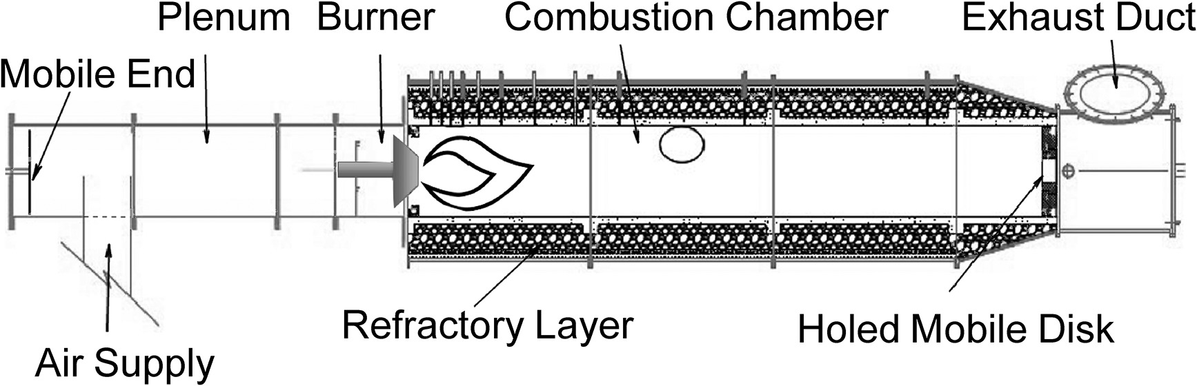
A thick layer of refractory is interposed between the chamber walls and the external liner to make the test rig adiabatic. During the experimental session, it is possible to control air and fuel mass flow rate, as well as air temperature and the length of plenum and chamber. The length of the rig can be continuously varied in order to tune the frequency at which combustion instabilities occur. Further details about experimental setup can be found in the study by 26.

Description of the numerical setup

The LES computational domain is formed by a fully unstructured mesh of 11852789 tetrahedral elements. The mesh is refined in correspondence of the flame and mixing regions; the time step is 4×10⁻⁸ s, resulting in a Courant number equal to 0.7.

In order to reduce the computational costs and to be able to use a finer mesh in the flame region, the LES domain is shorter than the real combustion chamber (about one third of the real length). This assumption is considered acceptable since the recirculation zones are located well inside the LES domain; the flame is located in the first third of the LES domain; there is no diameter variation inside the test rig.

Inlet and outlet boundary conditions are imposed using the non-reflecting Navier-Stokes characteristic boundary condition formulation to control acoustic reflection 24. All the other walls are set as adiabatic and modelled using a logarithmic wall-law condition.

Flame transfer function numerical calculation

Once LES of the reactive process is statistically converged, a specific procedure to compute the FTF is performed. A multi-sinusoidal signal is imposed as velocity component normal to the burner inlet 26. This signal is applied both at the diagonal and at the axial inlet to excite heat release oscillations. Velocity excitations normalised by the respective mean velocities are identical in the both diagonal and axial channels of the burner. When velocity perturbations pass through the blades of diagonal and axial swirlers, tangential perturbations of velocity are produced. The frequencies imposed in the multi-sinusoidal signal are chosen in a wide range of frequencies that permit to determine the shape of the FTF with reasonable accuracy and focused on the frequencies of interest of the industrial burner.

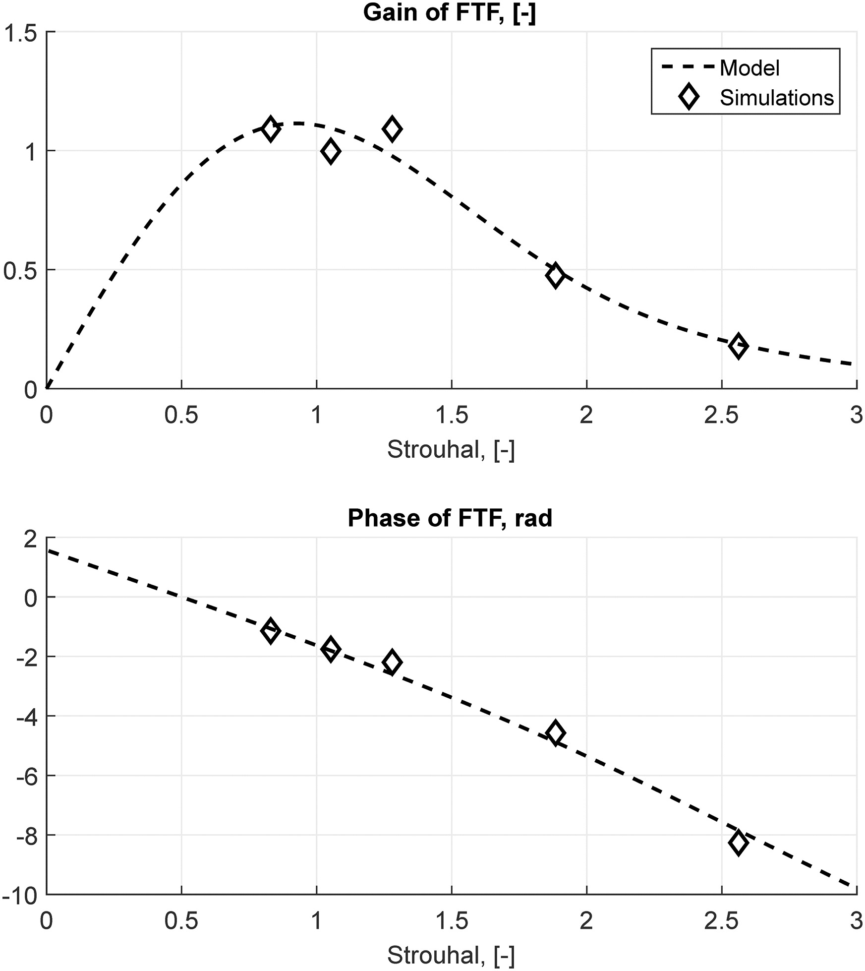
The velocity fluctuations are recorded by numerical probes. These probes are located both in the axial and in the diagonal passages, as shown in Figure 4. Specifically, the velocity fluctuations recorded by these probes have been normalised against their own average values. The heat release fluctuations are computed as a global value of whole combustion chamber. The simulation is run for a time to guarantee at least six periods of oscillations at the lowest frequency of excitation. Frequencies are reported in terms of Strouhal number, which is calculated taking the inner diameter of the combustion chamber and the average velocity at the exit of the burner as the reference length and velocity, respectively. The FTF is calculated for each frequency imposed in the multi-sinusoidal signal and is shown in Figure 5.

Figure 5.

Numerically computed FTF and the FTF modelled with (11).

Figure 4.

Schematic probes position for the FTF calculation 26.

Low-order network model setup

The numerical setup has been divided into six regions with three jump conditions with pressure losses, one jump condition at the flame and two boundary conditions as shown in Figure 6. The values of the cross-sectional area normalised against the cross-sectional area of the combustion chamber, the lengths of the sections normalised by the reference length and the temperature normalised by the temperature of the air at the inlet for each section are listed in Table 2. The jump matrices to connect acoustic waves between sections are calculated using (15) and (16). The reflection coefficient of the inlet is taken R_inlet. The outlet reflection coefficient R_out,1 is measured experimentally using multi-microphone technique. Several values of the outlet reflection coefficient around the measured one are tested in this study because of some uncertainties in this value, particularly caused by microphones cooling. The normalised total length of the combustor (sum of the lengths of Sections 5 and 6) is varied in the range L_c.c.=0.741÷1.593 with the step of ΔL_c.c.=0.037. Acoustic losses at area changes between plenum and burner and between burner and combustor are taken into account by pressure loss coefficients ζ_decr=0.442 and ζ_decr=0.718, respectively, calculated by the formulae proposed by 13. Acoustic losses at the swirler are obtained from the measurements. The active flame, i.e., the unsteady heat release, in the low-order network model is positioned at x_fl=0.1. This value corresponds to the maximum of the heat release in the longitudinal direction in LES. Mean temperature is uniform in the first five sections. The temperature gradient coincides with the position of the active flame and is situated between Sections 5 and 6.

Figure 6.

Scheme of network model numerical setup divided into sections.

Results of linear network model simulations

For each set of parameters, the simulation is run for 0.3 s that is enough to observe whether the pressure oscillations grow or decay in time. The setup is excited at the inlet for first t_exc=0.1 s by the broadband excitation in the range of Strouhal number 0÷7.53 with the maximum amplitude of the signal 5 Pa. After 0.1 s till 0.3 s, the system is left to evolve by itself without external excitations. We make use of a parameter called cycle increment that gives information about the thermoacoustic stability of the system. It is possible to calculate the cycle increment from the time-domain simulations assuming the following law for the pressure perturbations:

where f_i is one of the frequencies of pressure oscillations after t_exc, n is the number of the frequencies of pressure oscillations after t_exc, P_i is the amplitude of pressure oscillations at f_i at the time t_exc, θ_i is the phase of the pressure oscillations at f_i and α_i is the cycle increment of the mode f_i. Positive values of the cycle increment parameter α_i indicate that the system is unstable, and the negative values of α_i mean that the system is stable.

The frequencies of oscillations and their cycle increments are computed by approximating the time history of the pressure oscillations by (17) using the least-squares method. In the simulations presented in this study, either one or none unstable frequency per run is detected, thus n=1 for all simulations in the network model.

Dominant frequencies of pressure oscillations and their cycle increments for various lengths of the combustion chamber are shown in Figure 7. Frequencies are normalised with respect to the mean flow velocity at the burner exit and the diameter of the combustion chamber. The dominant frequency of oscillations decreases while increasing the length of the combustion chamber. This indicates the acoustic nature of the modes computed in this study. The calculated frequencies agree well with the experimentally observed frequencies.

Figure 7.

Dominant frequencies of the pressure oscillations and their cycle increments for various lengths of the combustion chamber.

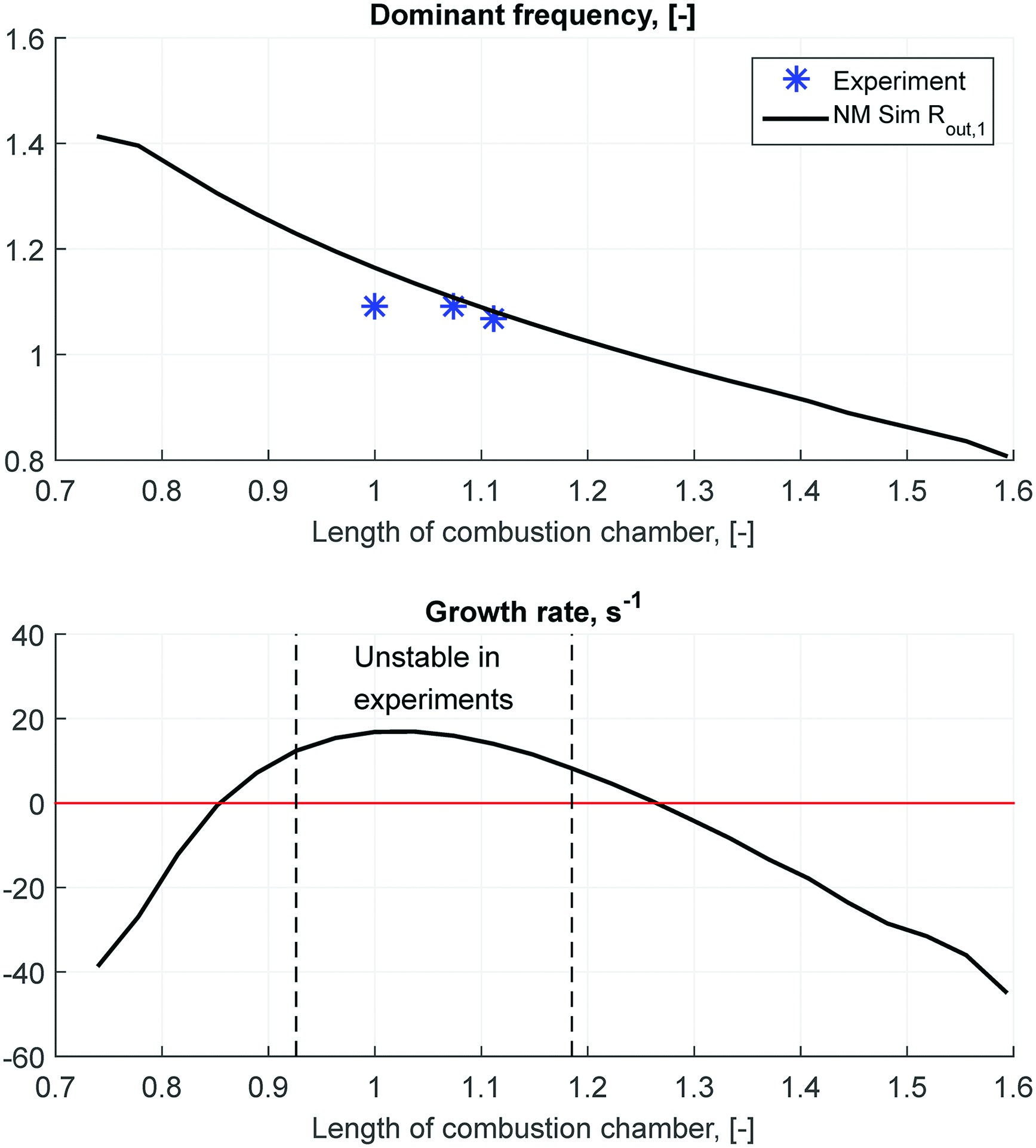
Thermoacoustic instabilities were observed in experiments in the range of combustion chamber length L_c.c.=0.93÷1.19. Simulations in the network model capture the unstable behaviour of the system qualitatively and predict the setup to be unstable for the slightly wider range of the values of the normalised combustion chamber length in L_c.c.=0.85÷1.30 (see Figure 7).

Results of weakly nonlinear network model simulations

It is possible to perform a weakly nonlinear analysis using the network model and the nonlinear heat release model. To do so, it is necessary to know the FDF — the response of the heat release to acoustic perturbations of different frequencies and different amplitudes. Since there is no available computed FDF of the setup, it is possible to mimic the nonlinear flame dynamics assuming the dependence of the parameters τ_i and σ_i on the normalised amplitude of velocity perturbations A upstream the flame. It was observed in a laboratory setup 14 that while increasing the amplitude of velocity excitation, the peak of the heat release distribution along the longitudinal axis was shifted towards the burner and the heat release distribution along the longitudinal axis became wider, i.e., the flame length was augmented. This means that when the amplitude of velocity perturbations upstream the flame is increasing, parameters τ_i are decreasing and parameters σ_i are increasing:

Square decay of τ_i parameters and linear increase of σ_i parameters gave smaller norms of residuals in 14 and are used in this study as well. Ratios of the second terms to the first terms of Equations (19a) and (20a) are taken the same as in 14. Absolute values of the second terms in Equations (19b) and (20b) are the same as in Equations (19a) and (20a), respectively.

When the amplitude of velocity perturbations approaches 0, values of τ_i and σ_i modelled by (18) and (19) approach values in Table 1, i.e., the FDF becomes the FTF computed by LES.

The network model setup is excited at the inlet by the same signal as in the linear analysis for first t_exc=0.1 s. After 0.1 s till 1.0 s, the system is left to evolve by itself without external excitations that is enough to reach either saturation to limit cycle pressure oscillations or infinitesimal pressure fluctuations. The maximum amplitudes of the pressure oscillations measured in the last 100 ms of simulations are plotted in Figure 8. Simulations are performed for the range of the combustion chamber length that are predicted to be unstable by the linear analysis and for three values of the outlet reflection coefficient R_out,1, 0.97R_out,1, and 0.94R_out,1.

Figure 8.

Amplitude of pressure oscillations for various values of the combustion chamber length.

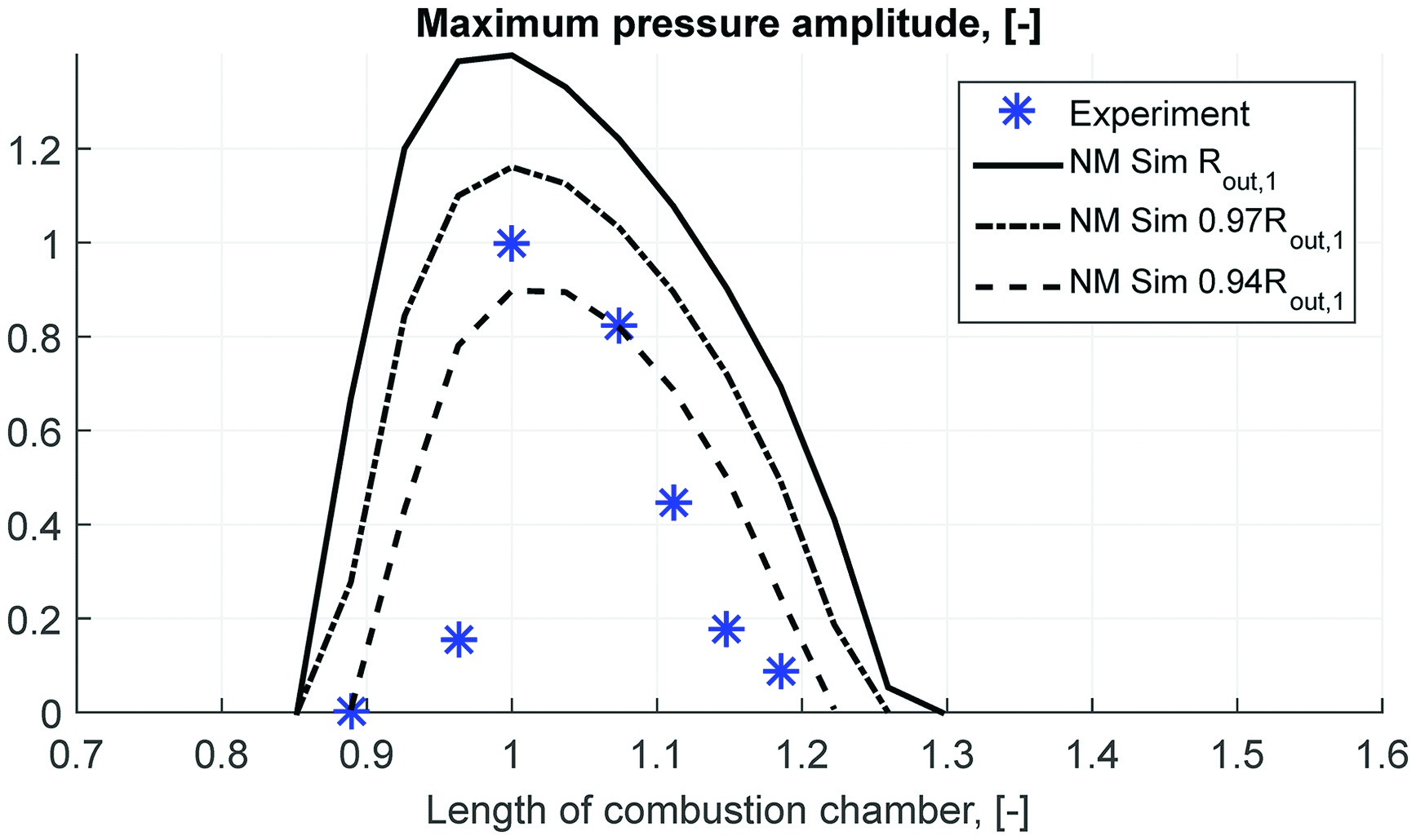
Unstable frequencies of the pressure oscillations in the weakly nonlinear analysis are the same as in the linear analysis shown in Figure 7. Nonlinear simulations capture well the trend of experimental dependence of the pressure oscillations amplitude on the length of the combustion chamber (see Figure 8) with the assumed nonlinear model of the FDF. Simulations employing the outlet reflection coefficient reduced by 6% with respect to the measured value give a good match with experimental data.