
Introduction
Rising competition as well as rising energy prices force engine maintenance repair and overhaul (MRO) provider to improve their overhaul process. Therefore, engine customers call for compliance of exact performance parameters like TSFC and EGT. To reach the given goals, MRO providers strive for condition based maintenance. Thereby, each engine receives customized MRO actions based on the engines history and operation to reach the given goals. To improve the engine performance with minimum effort, tailored repairs can be an option. Thus, detailed knowledge of wear and repair effects are necessary.
Focusing on HPC blisk maintenance, the MRO providers are faced with even more challenging tasks. Blisk blading cannot be re-arranged or replaced individually. Unfavored combinations of airfoils are to a much higher degree a given result of manufacturing tolerances superimposed by operation and repair.
The manufacturing tolerances are investigated by Lange et al. (2009, 2010, 2012). The result of these were a high influence of the thickness related parameter as well as the stagger angle on the loss coefficient. Also, Lange et al. (2012) carried out CFD simulations for non-axis-symmetric airfoils. Thereby, they simulated 1, 2, 4 and 8 passages. As a result, they showed that two simulated passages can have a higher negative influence on performance than one passage. Increasing the number of passages lead to increased spreading.
Blisk airfoil variations based on manufacturing tolerances are investigated by Backhaus et al. (2017). They showed that the milling of blisks lead to alternating geometric variances on the circumference. This alternating behavior is traced back to the abrasion behavior of the milling tool. The manufacturing process leads to a clustering of airfoils for unequal and equal circumferential positions. Reitz et al. (2014); Reitz and Friedrichs (2015); Reitz et al. (2016a, b); Reitz and Friedrichs (2017) are investigating the influence of geometric variations caused by wear. Therefore, two used HPC airfoil sets were scanned (e.g. Marx et al., 2013) and investigated. To rank wear parameter they performed a sensitivity analysis of a deteriorated HPC front stage by means of a DoE (e.g. Reitz et al., 2016b). As a result, they showed that the work coefficient Ψ and the pressure coefficient e are mainly effected by stagger angle, max. profile camber thickness and its position. Furthermore, the influence on loss coefficient ξR was investigated, which showed the leading edge geometry as the highest ranked parameter. In this paper the work of Kellersmann et al. (2017) is continued by investigating aerodynamic effects of deterioration. The focus of this study is the interaction of flow phenomena between two differently shaped airfoils. To limit the effects to geometric variations, quasi3D (Q3D) simulations of the 85% blade height are taken out.
Blisk wear
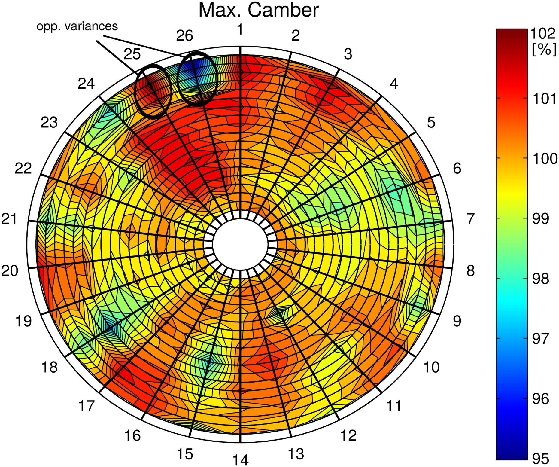
In order to determine the statistical background of degenerated and repaired airfoils, ten blisks, which are installed as a first stage in a HPC, are evaluated. The engine, a BPR = 5 turbofan engine is installed as a rear mounted engine mainly in regional and business aircrafts. Every blisk has been in operation for about 20,000 cycles. Each blisk has 26 airfoils which sets the statistical data to 260 blades. To gain geometric information about the blisks, each is scanned by a structured-light 3D scanner in conjunction with a photogrammetric system. This measurement technique results in a point cloud of the entire blisk. To achieve a good resolution quality, the measured volume of the 3D scanner is reduced from 170 × 130 × 130 mm for the blade to 80 × 60 × 60 mm at leading edge (LE) and trailing edge (TE). The resulting point density is shown in Figure 1. All blisk are cleaned before scanning so no depositions change the resulting point cloud. The geometric variances are gathered by an in-house programmed analyzing tool developed by Reitz and Friedrichs (2015). This analyzer evaluates the geometric properties of the point clouds of all airfoils on 19 2D-profile sections from 5% to 95% blade height. This process delivers the parameters listed in Table 1 for every 2D-profile. The geometric parameters are explained by Reitz and Friedrichs (2015) and in Reitz et al. (2018). To focus only on geometric variances of the blade profile, the hub and tip region are neglected, despite of their influence. As an example for the degenerated and repaired blisk, Figures 2 and 3 show the radial distribution of leading edge thickness for blisk 10 and in the same manner the max. camber thickness of blisk 7. The plots show the variation of the airfoils to a chosen airfoil of the statistical data representing a mean value. The maximum range of deviation is ΔtLE = 12% and Δcmax = 7%. Additional to the degeneration, a blend-repair can be detected at the LE of blisk 10, airfoil no. 24 (cf. Figure 3). But a more important aspect to be considered is the inhomogeneous wear on airfoils circumferential placed next to each other. This result shows the difference between geometric variations caused by manufacturing tolerances (e.g. Backhaus et al., 2017) and geometric wear effects because there is no alternating behavior. Also the comparison with Marx et al. (2013) shows a similar behavior for the wear pattern. Blisk 10 shows such combinations for the max. profile camber thickness (cf. Figure 2). Blades 25 and 26 have opposite variances as well as blade 17 and 18. Also for blisk 7 such arrangement (blade 8 and 9) is detected. With these examples it is shown that adjacent airfoils can have wear pattern which are influencing the aerodynamic behavior of their own and their neighboring ones. In Figure 4 the statistical distribution of the maximum profile camber thickness along the blade height is shown. The basis of this distribution are 10 blisk referenced to the chosen airfoil. It has to be mentioned, that no newly manufactured blisk could be analyzed. But the comparison with Marx et al. (2013) show, that the found wear distribution is in a same magnitude. The spread of the distribution has a maximum of 11% in the tip region, which is confirmed by Tabakoff (1987) as a region of high deterioration. The standard deviation for the considered blade-height is σ = 1.7%. This spreading is the base of the design space, which is used for the DoE.
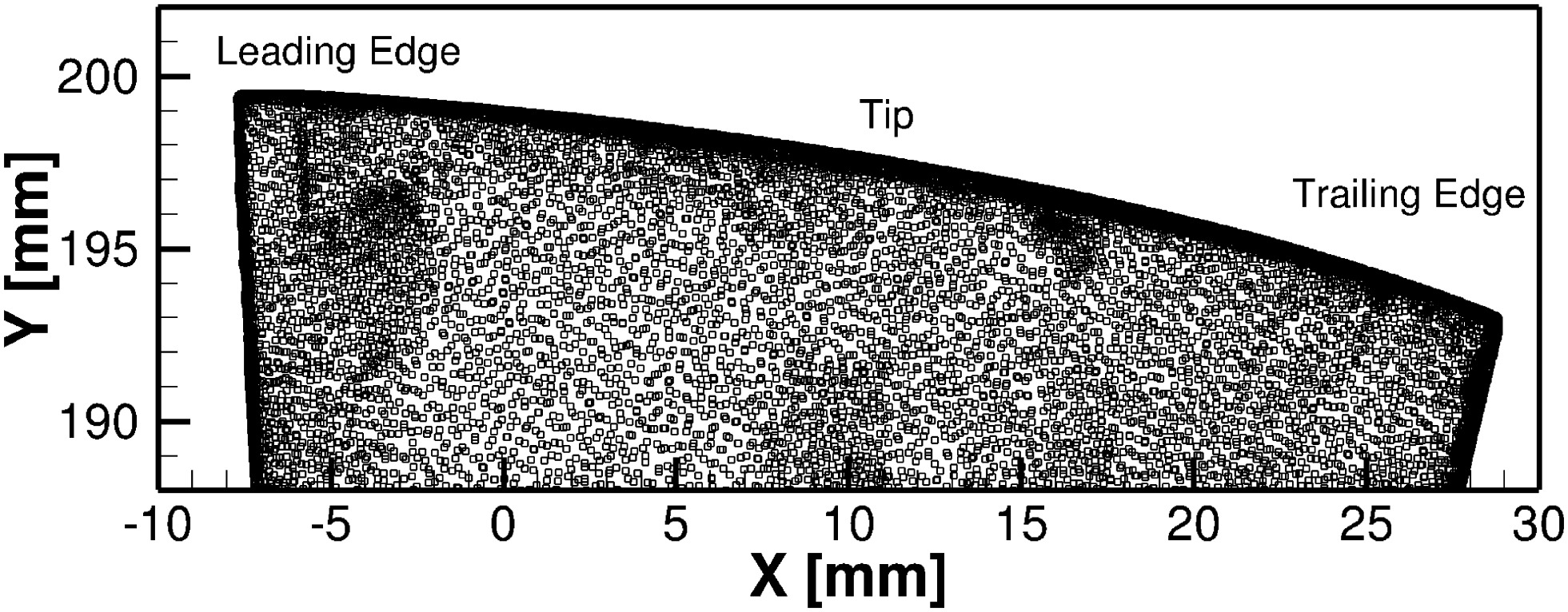
Figure 3.
Variation of max. camber thickness of 10 blisk blades expressed as a percentage of a reference value.
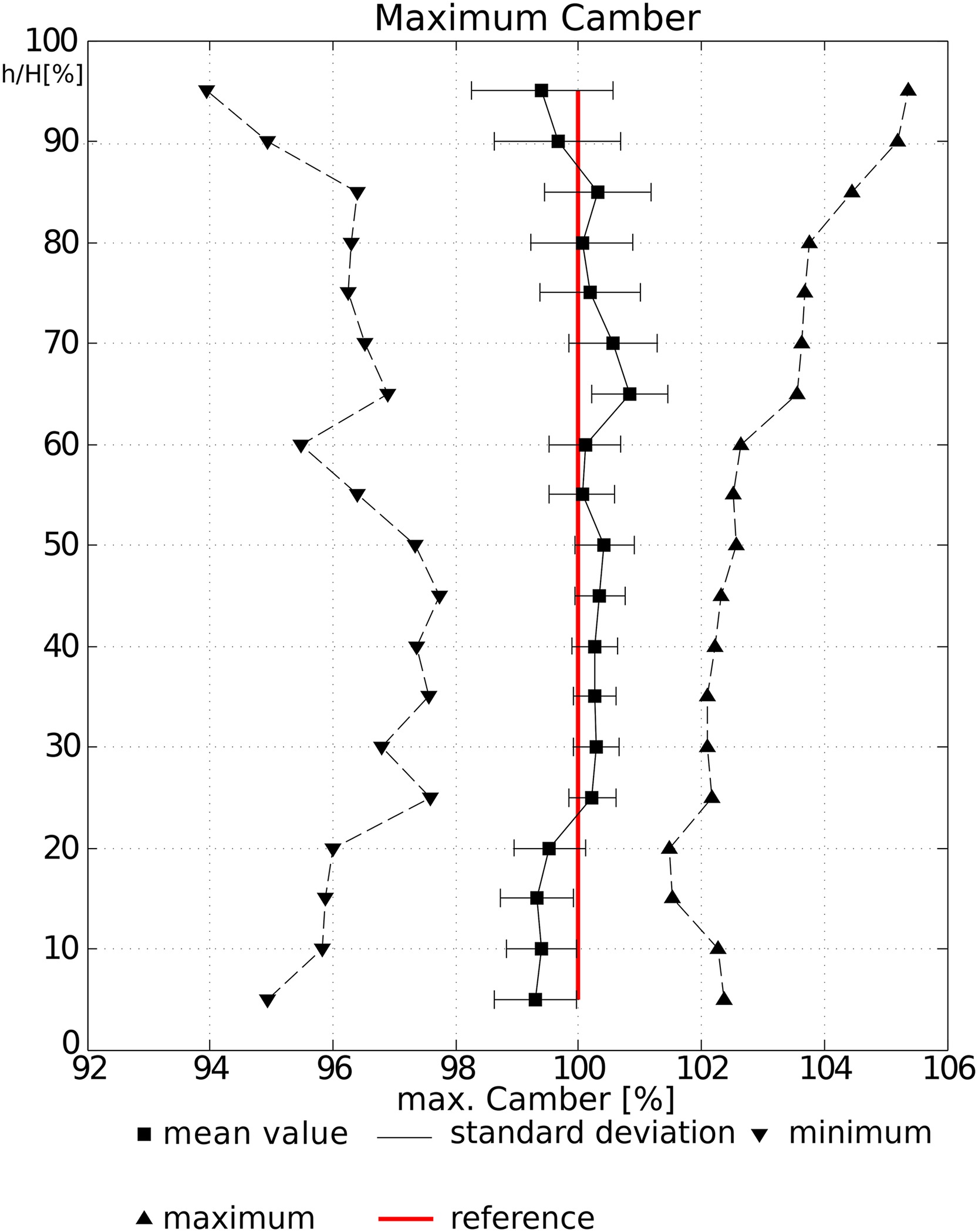
Figure 2.
Circumferential rotor blade leading edge thickness on blisk no. 10 expressed as a percentage of a reference value.
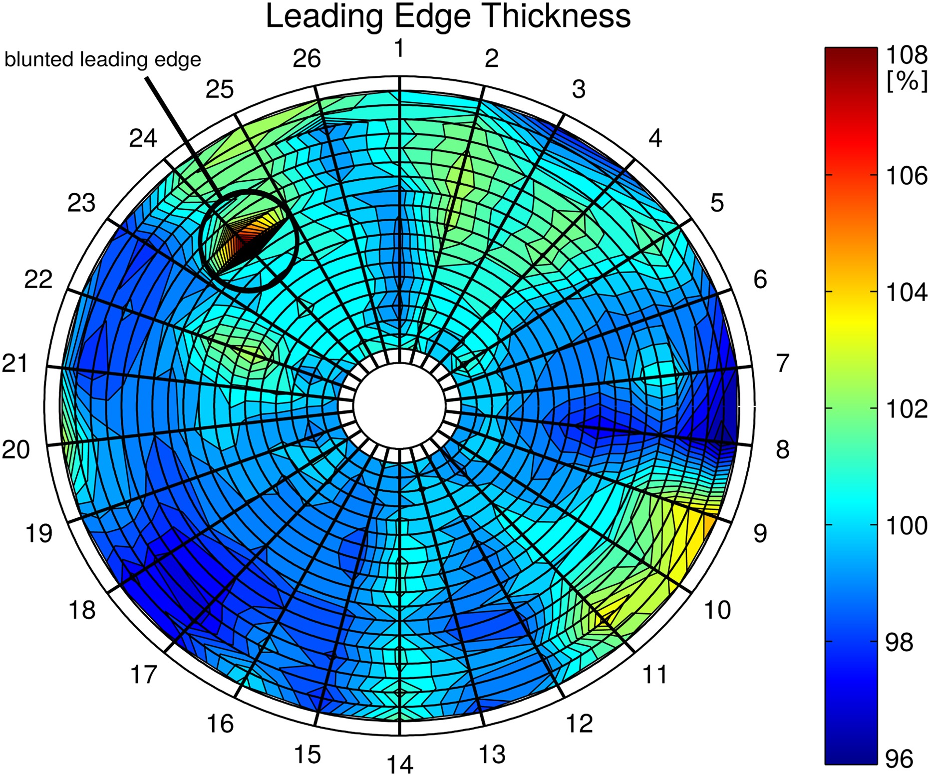
Table 1.
Investigated geometric parameters.
Design of experiments
In order to rank the influence of the wear pattern, a detailed DoE for front stage blisk-airfoil variations is done. The work of Reitz and Friedrichs (2015) is therefore extended through the focus on coupled deterioration effects and their interactions. The basis of the DoE is the 85% profile height section. This profile is chosen because the height is representative for a front stage blisk and the influence of the tip gap vortex is neglectable. It has to be mentioned, that due to a missing of a newly manufactured blisk a comparable front stage rotor blade well known to us, is the basis of numerical analysis. The transferability is given by comparison with Marx et al. (2013) whom investigated this front stage. The geometry is created by an in-house programmed algorithm developed by Reitz and Friedrichs (2015). To carry out a sensitivity analysis of the geometric parameters shown in Table 1, the rotor-airfoil profiles are modified in their geometric properties in a range of ±1.5σ, whereas σ is the standard deviation of the wear characteristics of the analyzed blisks shown in Figure 4. To reduce the number of parameters and to avoid mistakes during the DoE, correlations between geometric parameters have been taken into account. The correlations of the blisk wear pattern are investigated similarly to a process Reitz et al. (2016a) developed, which is based on the linear correlation coefficients of Pearson (1920) and Cohen et al. (2013). The coefficients are calculated by the covariance of the coupled parameters sxy and the covariance of the single parameters sx and sy (Equation (1)). This evaluation is done for the 16 measured blisk parameters and the following correlations were found.
The correlation coefficients 2 and 3 show a strong coherence between edge parameter at the LE and TE (Kronthaler, 2014). As described the parameter tLE defines the behavior of the LEstretch and the rTE. The same applies to the trailing edge. Thereby, the parameter LEstretch and TEstretch define a ratio of a length, which is 1% of the chord length with the thickness measured at 1% chord length (Reitz et al., 2018). If a thicker edge parameter appears, the edge stretching is decreasing. The stretching again provides higher radii. Thus, the correlation between the edge parameter reproduces blunted edges as well as sharpened edges. The correlations have two important functions. On the one hand, the parameter set for the DoE is reduced. Therefore, the number of training data set calculations is reduced, which in turn improves the meta-model. On the other hand, correlations in the meta-model are prescribed by before defined correlations. This also reduces the meta-model error. To train the meta-model, a data set of 700 data points is used. Each data point consists of 12 parameters for each blade. The data points are equally distributed by a Latin-Hypercube-Sampling algorithm of Lophaven et al. (2002). Through this process, an equally distributed parameter space with coupled two airfoil passages has been created and evaluated.
Computational method
As numerical solver the parallel CFD-solver TRACE of DLR Cologne has been used for this investigation. The CFD code solves the three-dimensional Reynolds-averaged Navier-Stokes equations on multi-block meshes by finite volume method, cf. Nürnberger (n.d.), Kügeler (2005), Marciniak et al. (2010), Becker et al. (2010). The discretization method for the convective fluxes is the 2nd order TVD upwind scheme of Roe (1981). The diffusive fluxes are discretized by a central differencing scheme. An implicit predictor-corrector time integration algorithm has been used for steady state simulations. As turbulence model, the two-equation k-ω-model of Wilcox (1998) with the stagnation point anomaly fix of Launder and Kato (1993) is used. To capture the rotational effects, an extension is implemented by Bardina et al. (1985). The inlet and outlet boundaries are applied after the method of Saxer and Giles (1993). The boundary layer transition is modeled by the two-equation γ-Reθ -model of Langtry and Menter (2009). This model evaluates the local flow features to facilitate natural, bypass and separation induced transition. The correlation constants used in the transition extension of TRACE are optimized for turbomachinery applications Müller-Schindewolffs et al. (2017). The boundary layer parameters are determined by integration of the velocity field perpendicular to the blade surface up to a point where the total pressure has increased by 99% of the whole defect Kozulovic (2007). The boundary conditions of the blades (Table 2) are no slip walls with hydraulically smooth walls, so roughness induced changes are not considered. The used numerical models are suitable for predicting the flow phenomena which appears on the investigated blade height. Bode et al. (2012) investigated the boundary layer development of a compressor cascade similar to the used blade profile, here. They showed a good agreement between the numerical results and experimental data.
Table 2.
Boundary conditions of the computational domain.
| Setting | Comment |
|---|---|
| pt1, Tt1, α1, Tu1, TLM1 | Extracted from 3D-rotor simulation |
| Operation point | Cruise |
| Walls | No slip walls, hydraulically smooth |
Meshing
The grid shown in Figure 5 is divided into two domains to capture the effects of both altered airfoils independently. Both domains consist of approximately 200,000 grid points each with a high resolution of the boundary layer. All no-slip boundaries have a dimensionless wall distance of the wall adjacent cells below y+ <1. A grid independence study is conducted which results in the given mesh. To reduce the computational effort, only one cell in span wise direction is used. To capture the stream tube contraction effects, a varying height has been adapted to the mesh. Depending on test case blade condition, the convergence of steady state simulations was achieved after 9000–14,000 iterations, which was characterized by relative difference of in- and outlet massflow of 0.02% within 2000 iterations.
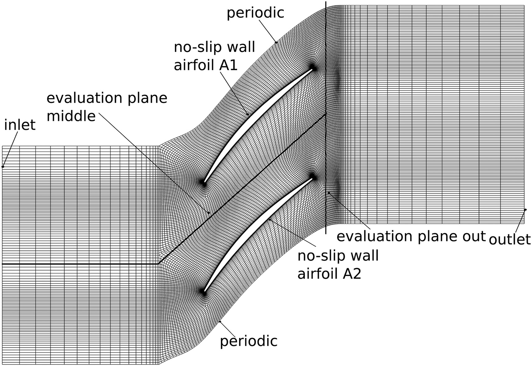
Adjustment of Q3D simulations
To ensure that the Q3D-simulations are in line with the 3D results, the boundary conditions need to be adapted. In Figure 6 the distribution of the AVDR (left) clarifies the influence on the passage. In the computational method, the influence of the AVDR is taken into account by specifying the Q3D stream tube height distribution. The method used is proposed by Stark and Hoheisel (1980). This method enables the Q3D simulations to reach similar results. Especially the boundary layer behavior and therefore a comparable pressure distribution can be reached. Along both parameters, the axial velocity density ratio (AVDR) has an influence on turning. This makes it possible to get the same influence of geometric blade variances as for a full 3D simulation, but with the advantage of detecting the fluid dynamic effects of coupled geometric wear parameters. The comparison of the pressure distribution, cf. Figure 7, shows a similar behavior but indicates that it is not feasible to exactly match Q3D and 3D simulations. The differences are due to the 3D effects of the flow around first stage airfoils. The tip near region of the airfoil shows influence of the tip clearance vortex as well as the contraction of the shroud. Both induce radial velocities which cannot be carried into the Q3D simulation. Furthermore, the evaluation plane is near the trailing edge, because a clear mapping of the resulting flow effects to the blade is necessary (cf. Figure 5).


Validation of meta-model
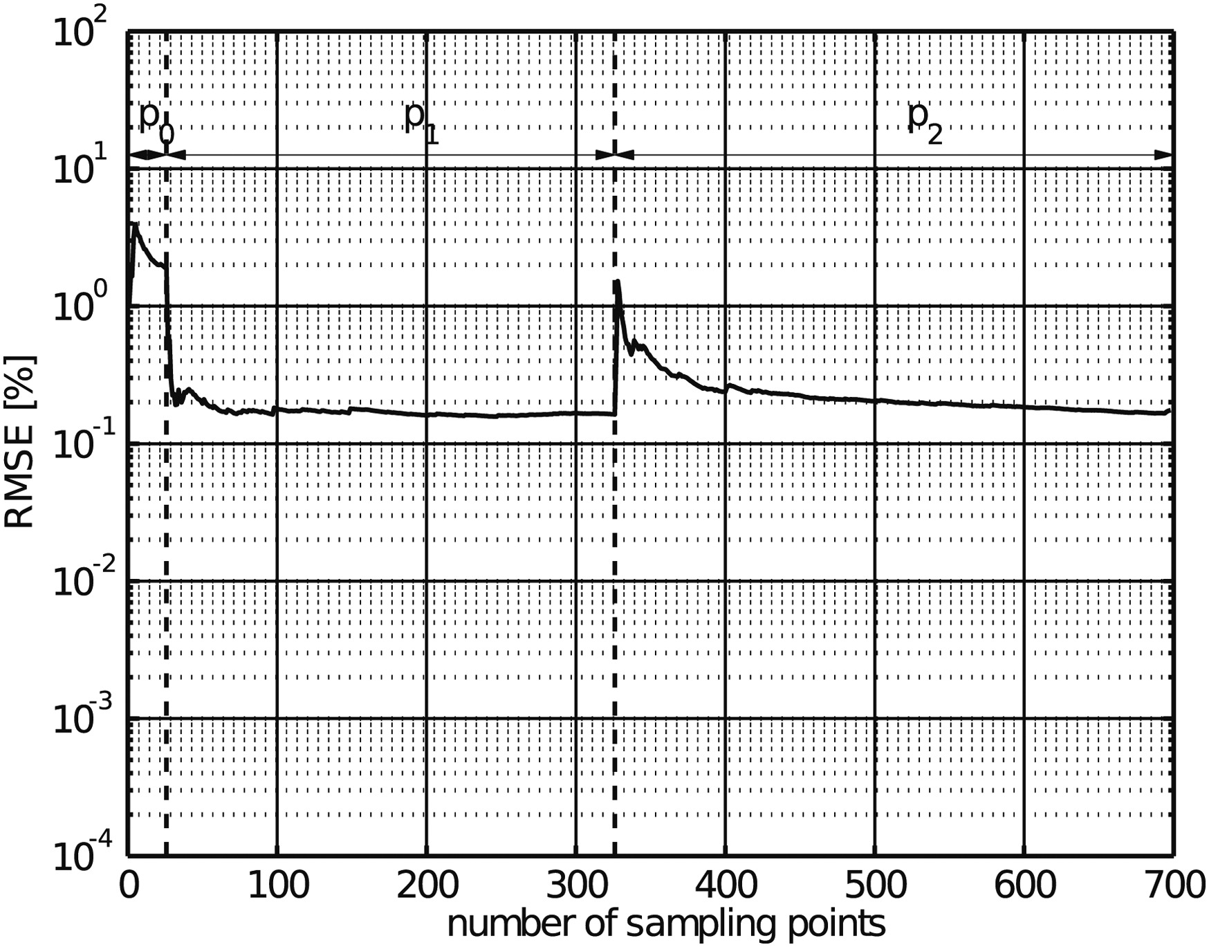
The Kriging-Method according to Lophaven et al. (2002) is used to generate a meta-model based on the DoE results of the CFD calculations. This meta-model, based on the design space of 700 samples, is used to generate Pareto charts to identify aerodynamic sensitivities of coupled wear parameters. To ensure the meta-model is working in a reasonable interpolation range the parameter range is limited between s independently. Thereby, the meta-model is trained in a valid parameter space. To validate the meta-model, the leave-one-out method is used. In Figure 8 the RMSE is shown for the prediction of the loss coefficient (Equation (4)). The chart can be divided into three subareas. The first, p0, shows the error with a constant prediction value for the Kriging-method. Here a high error of approx. 2% is calculated. For the second area, p1, the Kriging-method works on a linear interpolation and, as can be seen, the error is in a region of 0.2%. The third area p2 describes the error of the Kriging-interpolation working with a quadratic analysis. Here the error drop is slower but also reaches the region of 0.2%. This Kriging-method is best suited for the problem definition because it can be assumed that relations between geometric wear parameters and aerodynamic behavior cannot be mapped with a linear approach, cf. Reitz et al. (2016b). Through this validation, it is ensured, that the meta-model is able to predict the aerodynamic behavior of coupled airfoils.
Results and discussion
The aerodynamic performance of the airfoils is evaluated independently. In consideration of the massflow deflection of the flow field and the alternating characteristic both airfoils are divided into two domains (e.g. Figure 5) and each border with its specific massflow is taken into account. Thus, it is ensured that each airfoil is accounting for its effects. Both domains are analyzed by means of the loss coefficient ξ.
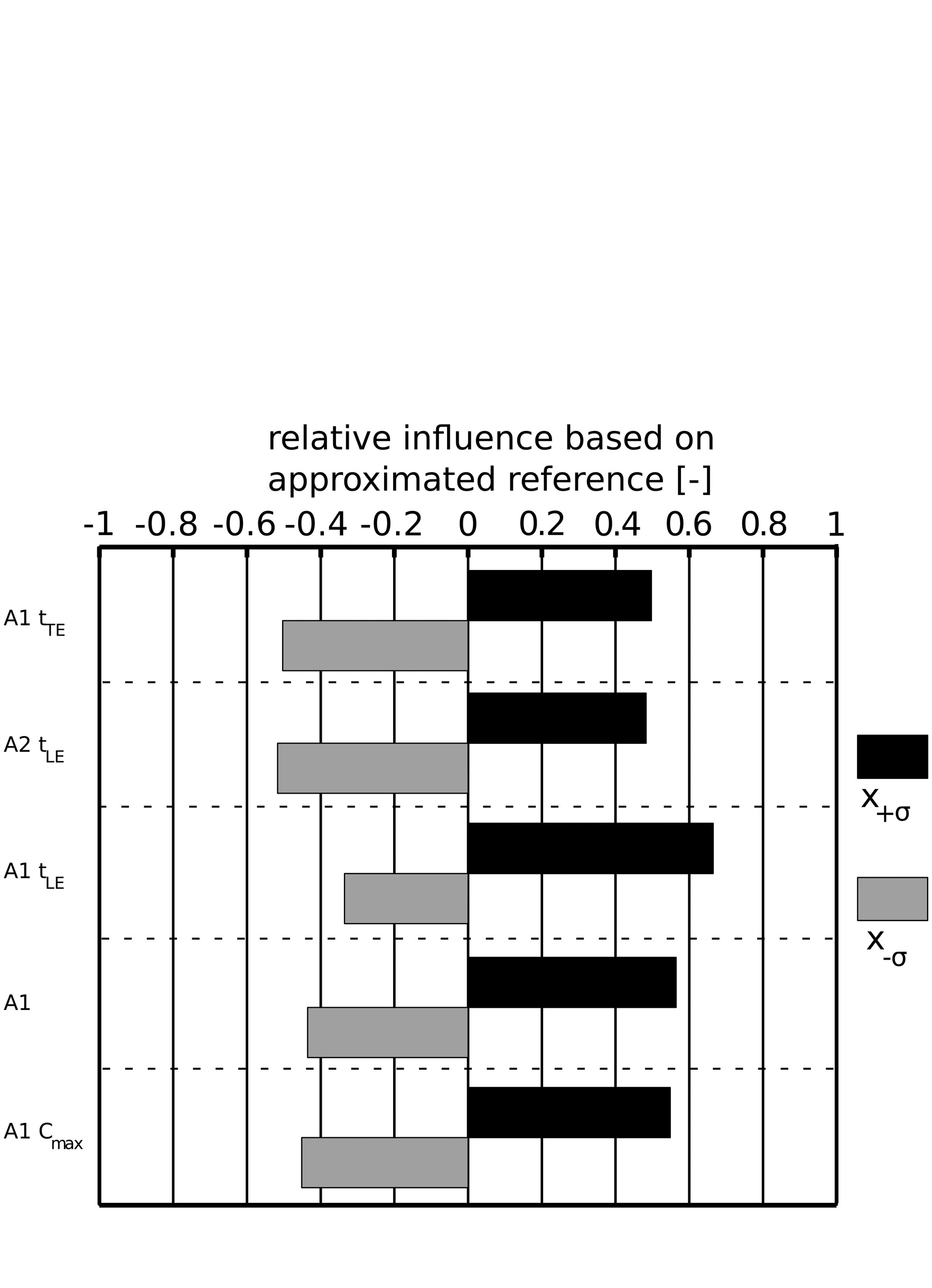
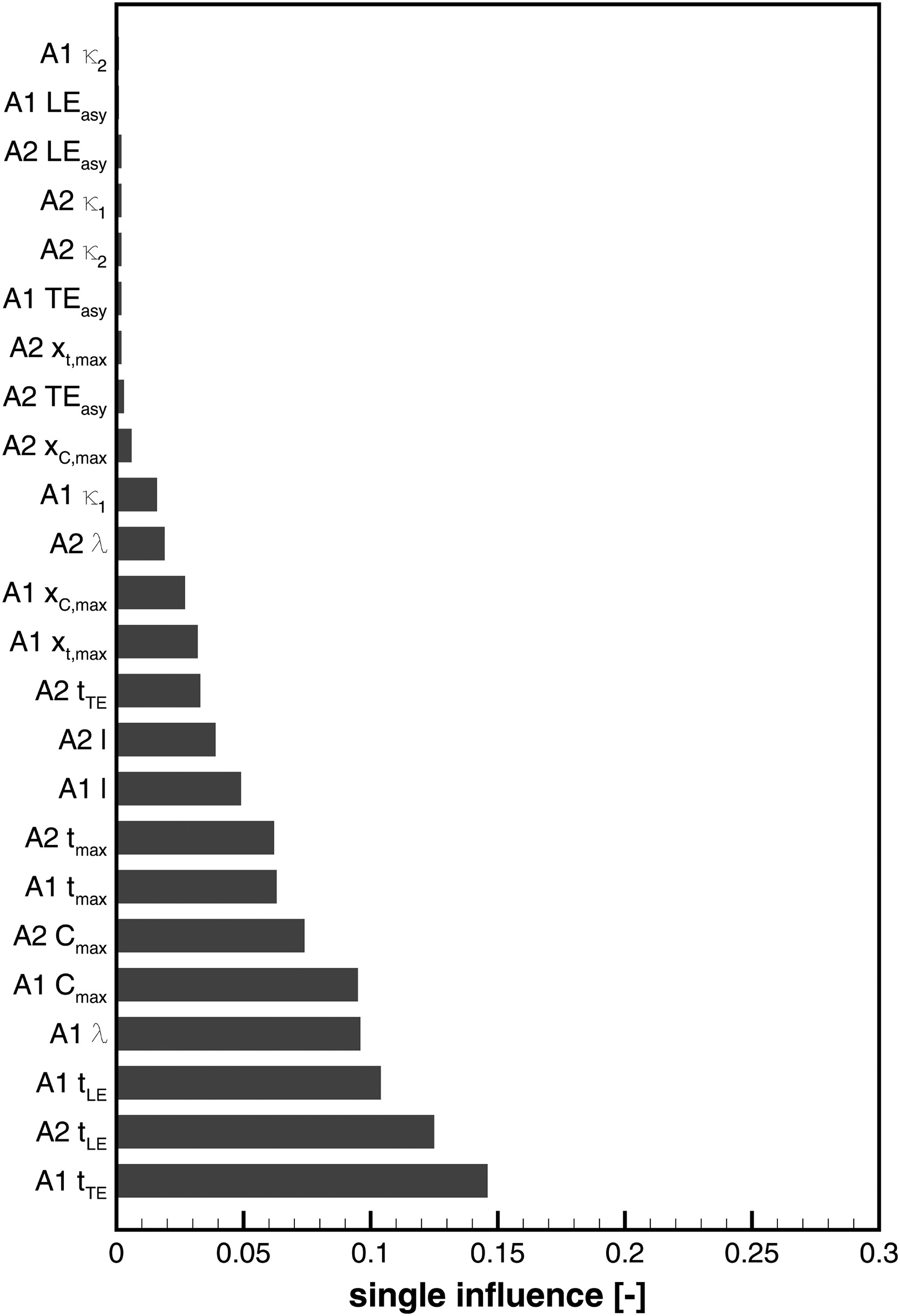
All parameters have been analyzed by the same boundary condition. As underlaying operating point of the compressor, cruise condition is chosen. To identify effects of coupled geometric properties, a Pareto chart and a sensitivity analysis of the corresponding parameters based on the design space are used. Figure 9 shows the Pareto chart for the loss coefficient ξ. The ordinate shows wear parameters of both airfoils (A1/A2) with an impact on airfoil A1. They are ranked according to their influence on the loss coefficient. Please keep in mind that the periodic boundary condition for the domain indicates an alternating blade arrangement. Therefore, the presumption is conservative in its consequence (e.g. Roberts et al., 2002). The six dominating parameters sorted by their influence are trailing edge thickness of airfoil A1, leading edge thickness for airfoil A2 and A1, the stagger angle of A1 followed by the max. profile camber thickness of airfoil A1 and A2. These six parameters represent approx. 64% of the overall influence. Looking at the single influence, leading edge thickness of airfoil A2, A2 tLE has a strong impact of 12.5% and thus a higher influence than the A1 tLE with 10.4% at the considered airfoil A1. Other parameters of airfoil A2 are A2cmax and A2tmax but both are ordered at position 6 and 8 with an influence of 7.4% and 6.3%. Compared to the work of Lange et al. (2010) and Reitz et al. (2016a) the ranking of wear parameter for the considered airfoil is the same. Only A1tTE is ordered in a higher rank than in the literature. This can be explained by using a profile section at 85% blade height. Using a Q3D-domain with an evaluation plane near the trailing edge, the effect of trailing edge thickness is overpredicted. Furthermore the mixing losses in the wake are neglected. Both leads to an overprediction, while Lange et al. (2010) and (Reitz et al., 2016b) used 3D blades with an evaluation plane downstream of the blades. In Figure 10 the sensitivities of the first five parameters are shown. The parameter A1tTE leads to greater losses with positive s as well as the leading edge thickness for airfoil A2 and A1. So raising edge thickness induces higher losses due to the increased wake and its blockage effects, not only for the considered airfoil but also for the adjacent one. Looking only at the losses of A1tLE, the impact of greater thickness is higher than of lowering it. This behavior is confirmed by Reitz et al. (2016b). In summary, the thickness related parameters as well as the stagger angle and the max. camber thickness have great impact on the performance of a profile. The leading edge thickness as well as the max. camber thickness distribution and the max. thickness have a significant impact on an adjacent airfoil. This indicates the sensibility of loss behavior to coupled wear parameters.
Fluid mechanical interpretations
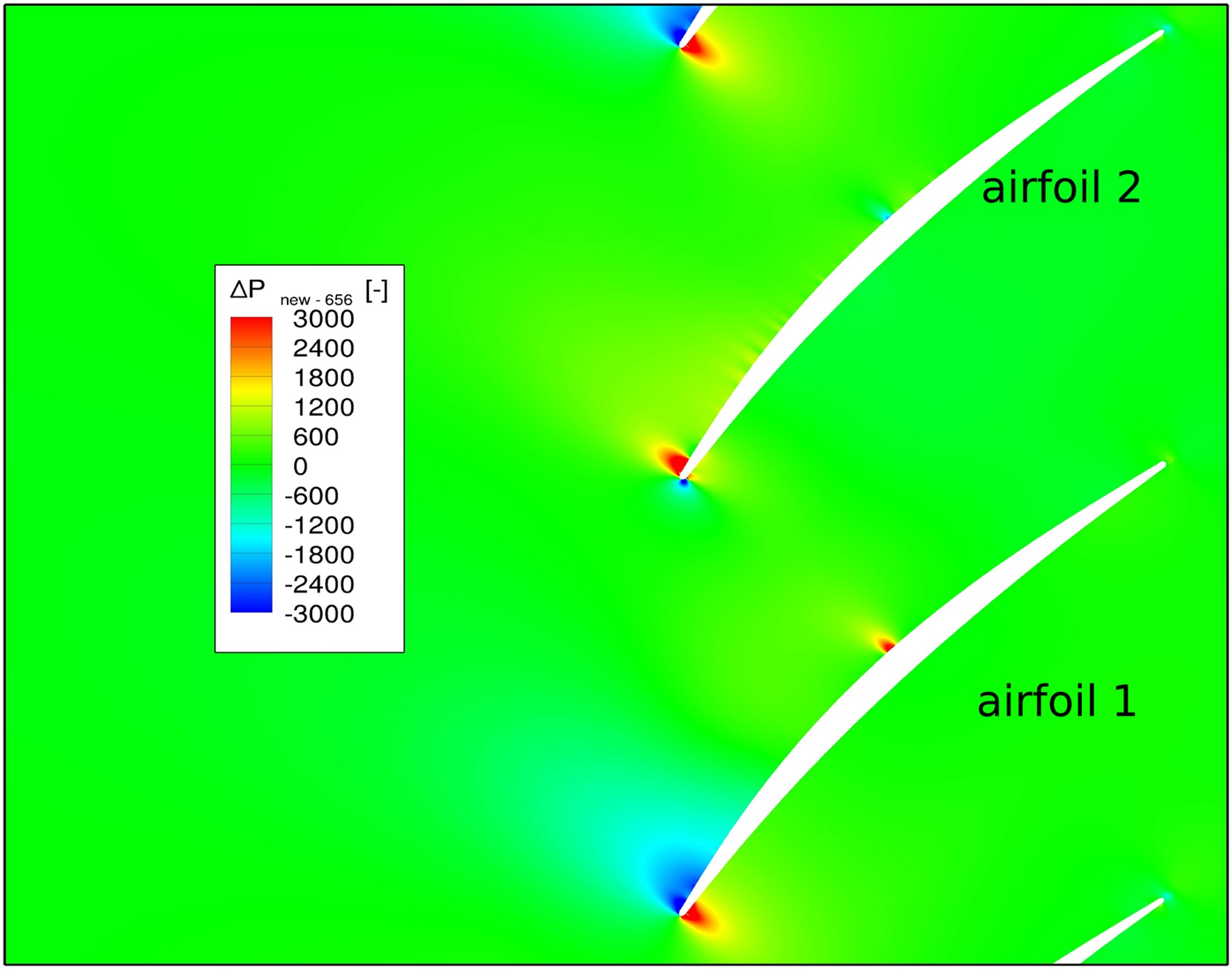
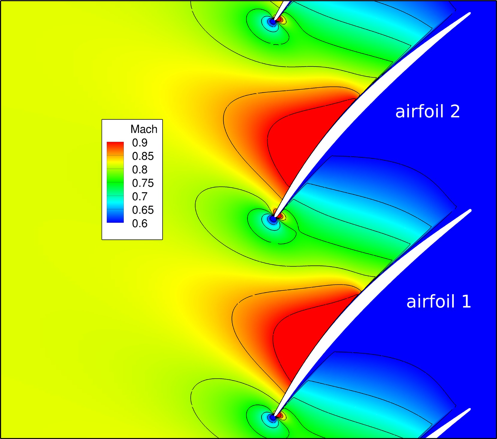
In order to further understand the fluid dynamics, design No. 656 is analyzed in more detail. The design No. 656 is an example for the interaction between coupled wear parameters (cf. Table 3) and have a strong impact on the loss coefficient. The shape of design No. 656 A1 is characterized by a high stagger angle (≈+1.5σ) and a low leading edge thickness (≈+σ). The adjacent airfoil A2 has a high leading edge (≈+1.5σ), a low stagger angle (≈−σ) as well as a low max. thickness (≈−σ) and a backward shifted camber thickness distribution (≈−1.5σ). This combination of wear parameters and interaction leads to the performance shown in Table 3. Therefore, the Mach number distribution of design No. 656 in Figure 11, the deviation of the pressure flow field in Figure 12 and the surface pressure distribution in Figure 13 are shown. The effects of differently shaped airfoils on the Mach number distribution are shown in Figure 11. The flow around the leading edge differs between both blades. A1 has only a small area of high Mach numbers at the leading edge whereas this area is stronger at A2. Furthermore the passage between the coupled airfoils is differently influenced. Both effects are related to the different shaped airfoils and their interaction. In Figure 12 the comparison of the pressure field from a new and the worn airfoil No. 656 is shown. Airfoil A1 has an area of lower pressure on the suction side of the leading edge and higher pressure on the pressure side in comparison with the flow field of a new airfoil. This can be related to the high stagger angle. This flow phenomena and the max. profile camber thickness leads to a shifted transition. Airfoil A2 has a thicker leading edge which results in a higher pressure on the suction side at the leading edge. To understand the consequence of the changed flow field, Figure 13 shows the cp plot for design No. 656 in reference to a new airfoil. The most distinctive wear effect is that the transition on the suction side of airfoil A1 is shifted towards the trailing edge. Furthermore, the loading of the airfoil is significantly reduced compared to the new airfoil. Also the leading edge is effected. Airfoil A2 has nearly the same pressure distribution as the new airfoil, but as depicted the leading edge is influenced. In Table 3 the performance parameter of both the coupled airfoils and their standalone simulations are shown. Looking at the flow turning a balancing for the coupled airfoils is detected. But for the pressure rise coefficient and the loss coefficient of the coupled airfoils a pronounced interaction can be seen. This behavior can be explained by the coupled geometric parameters. Looking at the Pareto chart of the loss coefficient (cf. Figure 9) confirm the effects of the coupled airfoils. Figure 14 compares the standalone pressure distribution of design no. 656 with the coupled simulation. Also here the standalone simulations show a slightly different behavior, which is related to their wear parameters. The point of transition for A2 is shifted towards the leading edge for the standalone simulation compared to the coupled simulation. For A1 standalone the transition is located behind the coupled simulations. The effects of the changed boundary conditions are also related to the interaction between the coupled airfoils. The stagger angle and the max. profile camber thickness connected with the leading and trailing edge parameters lead to the described effects. As can be seen in Figures 2 and 3 the circumferentially different wear can be detected in flown blisks. Thus, the simulated example can appear during operation of a jet engine. Furthermore, it can be assumed that coupled wear parameters can amplify each other due to a negative interaction of flow. Based on the evaluation of the DoE and analysis of the exemplary design no. 656, it is expected that coupled high ranked wear parameters like the max. camber thickness distribution, the stagger angle and the thickness related edge parameters increase the effects of wear. In summary the prediction of effects due to coupled wear and repair mechanisms can be explained by fluid dynamic behavior of the flow field and boundary layer changes.
Figure 14.
Comparison of the non-dimensional surface pressure distribution cp for design no. 656 and the standalone profiles.


Conclusion
The analysis of 10 measured blisks with each 26 airfoils of flown jet engines show significant geometric variances triggered by operation and regeneration. Furthermore, it can be seen that blisk airfoils wear differently on the circumference. In order to gain knowledge of the effects of coupled deteriorated airfoils on the aerodynamic performance on a high pressure compressor front stage, a DoE for the 85% profile section has been done. For the DoE, a parameter space of 700 different geometric designs using a LHS-method is created. These coupled airfoils are varied in the range of 1.5σ around the reference value of a new airfoil. These are processed by an automated algorithm to create the geometry and the mesh for the numerical steady state analysis. The flow of the Q3D airfoil simulations are adjusted to the behavior of the 3D-blade by using the AVDR, so a comparable flow behavior is ensured. The DoE shows strong dependencies between coupled wear parameters and performance.
a) On loss coefficient ξ only the leading edge thickness shows significant influence on coupled airfoils. A thicker leading edge leads to higher losses for the changed and also for the adjacent blade. The max. camber thickness and max. thickness are the next ranked parameters but have less impact. Other important parameters like trailing edge thickness and stagger angle only have a significant impact on the changed airfoil.
b) It can be concluded that high ranked wear parameters like max. camber thickness distribution, the stagger angle and thickness related edge parameters can lead to increasing wear effects. Based on the DoE the combination of A1tTE,+σ, A1tLE,+σ, A1λ+σ, A1cmax,+σ and A2tLE,+σ has a great impact on the loss coefficient. Within these coupled parameters an increasing effect of wear is expected.
In summary, a significant impact of wear parameters on adjacent airfoils can be detected. This result is supported by a view on the flow field changes and the surface pressure distribution. The flow field deviations are in a magnitude which have an influence on the adjacent airfoil and, therefore, change the performance. It was shown that wear parameters with a great influence according to the DoE have a great impact on the flow field and on the surface pressure distribution. Especially a change of the transition region has an influence on the loss behavior as well as a change of loading. All in all it was shown that a change of airfoil parameters due to wear not only change the performance of the considered airfoil but also have an influence on the adjacent airfoil. Also, there is the possibility that unfavorably coupled parameters occur during operation or maintenance and, therefore, the impact of wear and repair is strengthened. To apply the results to other blisk geometries, the important factor is a similar flow characteristic based on the geometric parameters. An exception are super-critical profile sections with supersonic incoming flow. Here the change of shock systems are highly relevant. Nevertheless, the gained knowledge of the interaction between different shaped airfoils due to different wear mechanisms improve the maintenance actions, especially for blisks.
Nomenclature
Latin
cp
Non-dimensional pressure coefficient, (p - pin)/(pt,in - pin)
cmax
Maximum profile camber thickness
h
Blade height
l
Blade chord length
LEasy
Leading edge asymmetry
LEstretch
Leading edge stretching
Ma
Mach number
p
Pressure
Re
Reynolds number
rLE
Leading edge radius
rTE
Trailing edge radius
tLE
Leading edge thickness
tTE
Trailing edge thickness
tmax
Maximum profile thickness
T
Temperature
TEasy
Trailing edge asymmetry
TEstretch
Trailing edge stretching
xtmax
Position of max. profile thickness
xcmax
Position of max. profile camber thickness