
Introduction
Increase in overall efficiency of aeronautical engines and stationary gas turbines, reducing specific fuel consumption, is being extensively researched. Since traditional engine configurations are reaching saturation development state, novel technological breakthroughs are sought. Among these radical changes, the most significant tackle either the core/bypass flows or the combustor losses. To address core flow hurdles, intercooling, Rankine bottoming and recuperation might be viable options. Reheating is also particularly developed for land-based applications. Concerning bypass losses, geared turbofan and open rotor concepts are receiving considerable attention (Grönstedt et al., 2013, 2016; Gülen, 2017).
With respect to the combustion losses, several innovative approaches have been proposed. Most of them aim at improving current constant-pressure (in fact, pressure-loss) combustion with a pressure-increase process. This so-called pressure gain combustion (PGC) can be accomplished by different means. The leading paths are pulse detonation (Roy et al., 2004; Pandey and Debnath, 2016), rotating detonation (Zhou et al., 2016; Kailasanath, 2017; Paxson and Naples, 2017), wave rotors (Akbari and Nalim, 2009; McClearn et al., 2016) and shockless explosion (Bobusch et al., 2014; Reichel et al., 2016) combustion. Some other concepts are the piston topping (Kaiser et al., 2015) and the nutating disk (Meitner et al., 2006). All these setups are theoretically supported by substantial thermodynamic gains, described in detail, e.g., by (Heiser and Pratt, 2002; Gray et al., 2016).
Despite fairly different construction and engine-integration characteristics, all these PGC processes introduce additional unsteadiness into the adjacent turbomachinery components, namely, the compressor upstream and the turbine downstream. This unsteadiness is directly linked with the inherently periodic nature of the combustion mechanisms, and affect the operation of both stationary and rotating parts (traditionally designed by steady state workflows). The integration between combustion units and engine (most likely through plena interfaces) is key to estimate proper boundary conditions for the neighboring components, such as perturbation signatures, operation frequencies and amplitudes.
Although fundamental combustion research on pulse detonation had been restricted to low frequency processes, massive increase in the number of ignitions per second has been achieved. Kilohertz pulse detonation frequencies were recently reported by (Taki et al., 2017). As for rotating detonation, it already takes place in the few kilohertz range (Lu and Braun, 2014; Bluemner et al., 2018). Similar periodicity is reported for the other PGC devices. This frequency range is also expected to be pushed up, once PGC technology takes off.
With respect to the amplitudes of such disturbances, they are strongly linked to the PGC operation (such as filling, ignition and purging phases), but also to the plena interfaces. Limited PGC experimental data with upstream measurements is available, such as (Roy et al., 2004; Rasheed et al., 2005). Some numerical work used pressure amplitude values at the combustor interfaces of a few percent up to approximately 40% (Van Zante et al., 2007; Fernelius, 2017; Liu et al., 2017). This disturbance amplitude range is already significant from the turbomachinery point of view, justifying detailed investigations.
The need for assessing the performance and aeroelasticity effects of these disturbances has been recognized by the combustion and turbomachinery academic community (Kailasanath, 2003; Roy et al., 2004; Rasheed et al., 2009; Lu and Braun, 2014; Gülen, 2017). However, quantitative information to evaluate the extent of these changes is scarce, especially for state-of-the-art industrial machines. Up to the current date, there has been no full integration between those PGC cores to commercial engines. Therefore, the current exploratory research sheds some light into the effects of this interfacing (specifically upstream), by numerical means. Both performance and aeroelasticity assessments will be presented.
The manuscript is organized as follows. In the case description section, the simulated high pressure compressor geometry is characterized. Next, the numerical methodologies both for the computational fluid dynamics (CFD) and computational solid mechanics (CSM) are presented. Subsequently, results are given for a broad range of disturbance amplitudes and frequencies, followed by the main outcomes.
Case description
A modern industrial high pressure compressor, depicted in Figure 1 is here used for the simulations (Klinger et al., 2008, 2011). Practical 3D geometries and operation points have been provided by an industrial partner. It is important to say that the whole engine has been designed for traditional deflagration combustion, without specific considerations for PGC and its effects on turbomachinery components. Therefore, the present study analyzes how this traditional setup would potentially react to unsteady disturbances and depart from the reference design.
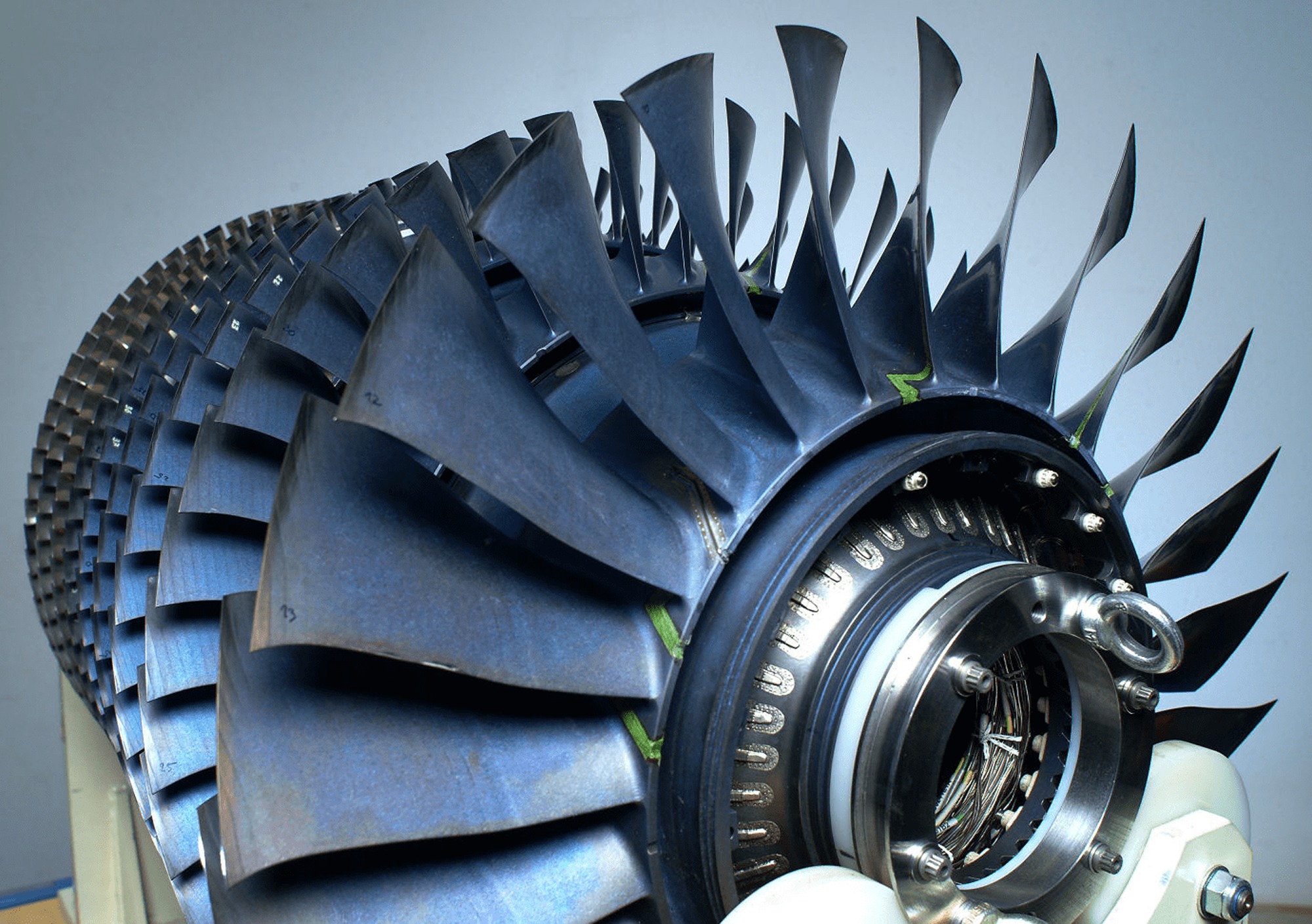
The simulated domain is the HPC 6th stage, the last with a bladed disk (blisk) design. Although it is not the very last stage right before the combustion chamber, it has been chosen considering that blisk manufacturing becomes increasingly more common in axial compressor design (Peitsch et al., 2005; Honisch et al., 2012; Mayorca et al., 2012; Zhao et al., 2015). Due to confidentiality constraints, the speedline itself and some absolute design quantities will not be disclosed here, but rather normalized values, enough for full comprehension and comparative evaluations.
Numerical methodology
For brevity purposes, neither the fluid nor the solid domain state and constitutive equations will be derived here. Rather, focus will be given to the interface treatment of necessary aeroelastic quantities, such as aerodynamic work or pressure harmonics. The next sections describe respectively the CFD (steady and unsteady) and CSM methodologies used along this work. The space and time independence studies for the grids are likewise presented.
Computational fluid dynamics
Due to the unsteady behavior associated with the new combustion processes, 3D unsteady viscid fluid dynamics simulations are employed, both in time and frequency domain. Time-domain calculations are here used to determine performance parameters, unsteady damping and blade surface pressure harmonics, to be later used in the structural simulations. Frequency-domain runs determine the aerodynamic damping.
(i) Steady state: the Navier-Stokes equations are boundary-layer resolved with the finite volumes solver CFX® (ANSYS Academic Research, Release 18.1), with air (ideal gas) as compressible medium. Fourth-order Rhie & Chow smoothing is employed (Rhie and Chow, 1983), while Reynolds stresses are computed by the two-equation Menter’s SST turbulence model (Menter, 1994). Since the simulated stage is located substantially far from the engine inlet, the flow is safely assumed to be fully turbulent, so no transition models were shown necessary. Double-precision, properly converged steady state solutions (with root-mean-square residuals lower than 10−5, and imbalances lower than 5·10−6) are used as initial conditions for the unsteady runs.
The 3D geometries were meshed with AutoGrid5® developed by Numeca (IGG™/AutoGrid5™ v11.1). Both root fillet and tip gap have been modeled. Multi-block structured hexaedra meshes were employed, with directional boundary-layer refinement on all walls (dimensionless wall distance
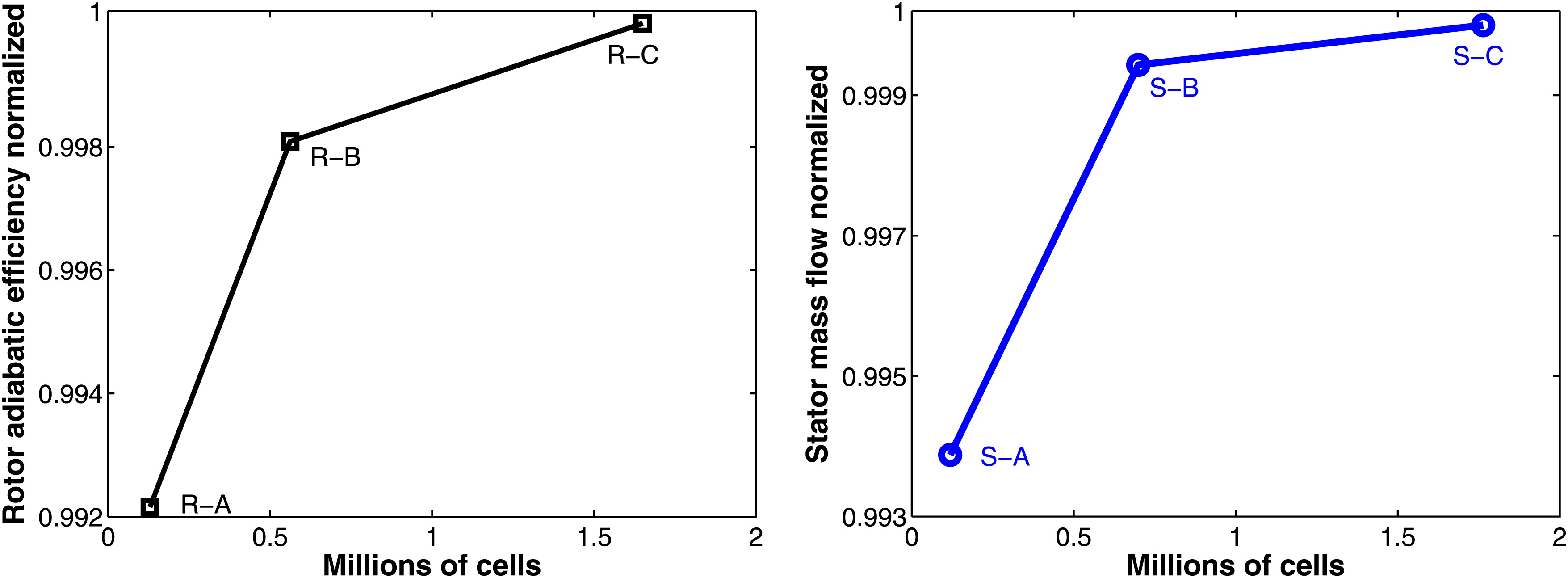
Several meshes were generated in order to perform a proper grid independence study, done separately for rotor and stator. The grids were refined as uniformly as practical, however always keeping the boundary layer on the walls resolved. Figure 2 displays three chosen meshes for rotor (labeled from coarsest to finest as R-A, R-B and R-C) and stator (labeled as S-A, S-B and S-C), with isentropic efficiency and mass flow values normalized by the finest grid, as a function of cell count. The deviation between the finest- and coarsest-grid values is less than 1% for both domains, in the sense that all displayed grids capture the global flow behavior accurately enough. The Grid Independence Index (Celik, 2008), formally derived based on the Richardson extrapolation (Roache, 1994), has been calculated and showed no oscillatory behavior. For the isentropic efficiency, the index between finest and medium meshes is GCIBC = 0.24%, with apparent order of 1.94. The grids utilized for the current stage are assembled together and shown in Figure 3. The number of nodes for the stage (if using one passage for rotor and one for stator) is approximately 1.3 million.
Figure 3.
Grids R-B and S-B for the simulated stage (rotor on the front and stator on the back), obtained after grid independence study. Geometry is rescaled.

As inlet boundary conditions, total pressure and temperature along with flow direction are implemented, while on the outlet the static pressure is prescribed. Both on inlet and outlet, radial profiles experimentally validated by the manufacturer are utilized. For the steady runs only, mixing-plane interface, with constant total pressure (that is, no loss in through the interface), is used to account for the non-unitary pitch ratio.
(ii) Unsteady: two types of time-resolved simulations are performed, with and without the PGC disturbances. The time discretization scheme utilized is the second order backward Euler, with a bounded high-resolution discretization for advection and viscous terms. The solution is deemed periodically converged when the relative difference between two consecutive periods for some globally integrated parameter (such as compression ratio or efficiency) or pressure probe falls below 0.05%. The attainment of quasi-convergence depends not only on the blade passing frequency (BPF), but also on the combustion-originated frequency and intensity, which in turn determines the required total run time.
The time resolution must be properly chosen to model the necessary phenomena without excessively consuming computational resources. For the present case, the main (a priori known) frequencies to be modeled by the time march are the rotor BPF and the disturbance frequency. A temporal resolution study was performed to determine the minimum time discretization required, using the number of time steps per rotor passing period (TSRPP) as a parameter. Pressure time traces of two points located between rotor and stator (one in each domain, respectively P1 and P2) are shown in Figure 4 (after periodic convergence is achieved). For both domains, 50 TSRPP are enough to accurately capture the unsteady behavior. To enhance resolution for the disturbed runs, a slightly higher value of 55 TSRPP has been chosen.
Figure 4.
Pressure probe periodically converged time trace, on rotor (P1) and stator (P2) domains. Several values for time steps per rotor passing period (TSRPP) are shown.

It is important to highlight that, under unsteady disturbances (additional to the rotor-stator frequency), the required time step could become smaller. To assess whether 55 TSRPP is enough for the outlet disturbance with the highest frequency here simulated (3.0 times the BPF), an extra run with halved time step (i.e., 110 TSRPP) was carried out, for an extra full rotor revolution. In comparison with the 55 TSRPP setup, a relative difference of 0.09% and 0.005% for isentropic efficiency and compression ratio, respectively, was found. Unsteady damping, as well as modal forcing (both defined further), showed similar minimal changes. From that, the current time resolution was deemed enough within the simulated disturbance range. Higher frequency disturbances could possibly require further time step refinement.
For the transient calculations, the number of rotor blades was reduced by one unit, so that 3 rotor passages and 4 stator passages yield a unitary pitch ratio. This modification prevents phase errors which would incur when using for example the profile-scaling method (Galpin et al., 1995). Time-inclining or -shifted methods, such as (Giles, 1988) or (Gerolymos et al., 2002), are not physically consistent when disturbance frequencies different from the BPF are present in the system. In summary, the current unsteady simulation setup does not induce frequency or phase errors due to non-unitary pitch ratio, with sliding meshes accurately modeling the transient phenomena that takes place between rotor and stator. All unsteady disturbances are modeled by the time marching scheme without further simplifications. The total number of nodes for this setup is approximately 4.6 million.
To model the PGC disturbances, time periodic boundary conditions at the stage outlet have been implemented. To the knowledge of the authors, no effective test rig or prototype coupling industrial axial compressor and turbine to a pressure gain combustor has been built, in a fully coupled fashion. Ongoing investigations focus on how to connect these components through adequate plena geometries, to minimize unsteadiness and therefore prevent extra losses. Accordingly, due to the lack of more precise plenum information, it is assumed that the unsteadiness reaching the compressor/combustor interface does not vary circumferentially, being here described by harmonic fluctuations, as in Equation (1).
Here,
(iii) Time-spectral: the frequency-domain method employed here is the nonlinear harmonic balance (Hall et al., 2002) (also known as time spectral method (Gopinath and Jameson, 2005)). The time and spatial dependent state variables are written as a Fourier series for a predetermined fundamental frequency, whose first harmonics are iteratively and simultaneously solved with a pseudo time march. Along this work, 3 harmonics (producing 7 time levels) have been used, after parametric studies showed that more harmonics did not change the solution substantially. Additionally, 20 pseudo time steps per oscillation period were enough to achieve the desired computational accuracy at rapid convergence. The nonlinear harmonic balance is here utilized to determine the aerodynamic work
Here, p is the static pressure,
With this approach, extensively used in industrial design, two assumptions are implied: constant vibration frequency (for each natural mode) and independence between damping and forcing (justified, for example, by (Mao and Kielb, 2017)). It is important to remark that the main vibration damping contribution for a blisk structure comes from aerodynamic forcing, since friction damping is not present, and material damping is negligible. Therefore the need of precisely determining the aerodynamic work on the rotor blade.
The aerodynamic work is used to compute the damping ratio
Here,
The time-spectral analyses simulate the rotor domain only, with the same inlet boundary conditions as for the stage runs (total pressure, total temperature and flow direction). Regarding the rotor outlet, design static pressure radial profiles for the corresponding axial position (validated by the manufacturer) are employed.
In this work, the rotor blades (which in general are under more mechanical stresses than the stator) vibrate on the first three natural frequencies (the most energetic, sufficient for aeroelastic structural response (Silkowski and Hall, 1997; Piperno and Farhat, 2001; He, 2010)), with a maximum tip displacement set to 0.5% of blade height. The normalization provided by Equation (3) makes sure that the damping ratio is independent of the chosen scaling factor q, within the quadratic regime. Parametric simulations have confirmed that the chosen values for the scaling factor and natural frequencies lie within the proportionality range expressed by Equation (3).
Computational solid mechanics
(i) Prestressed static and modal analyses: the current rotor blisk is modeled as a cyclic symmetric sector, with a typical modern industrial titanium alloy. Here, focus will be given to the blade geometry and mesh, sufficing to say that the disk displacement is fixed at the bore, that is, shaft flexibility is ignored, as standard with blisk analyses (Sever, 2004; Li et al., 2016). In the prestressed static analysis, constant rotational velocity and the mean static pressure on the blade surface are prescribed as loads. The pressure load comes from CFD-only simulation without any external disturbance, that is, a baseline unsteady run. The nodal pressure time history on the blade surface is expanded into a Fourier series, whose first term correspond to the mean static load (which is used in the prestressed static analysis). The following terms determine the engine order multiples (these shall be later used in the harmonic response analyses).
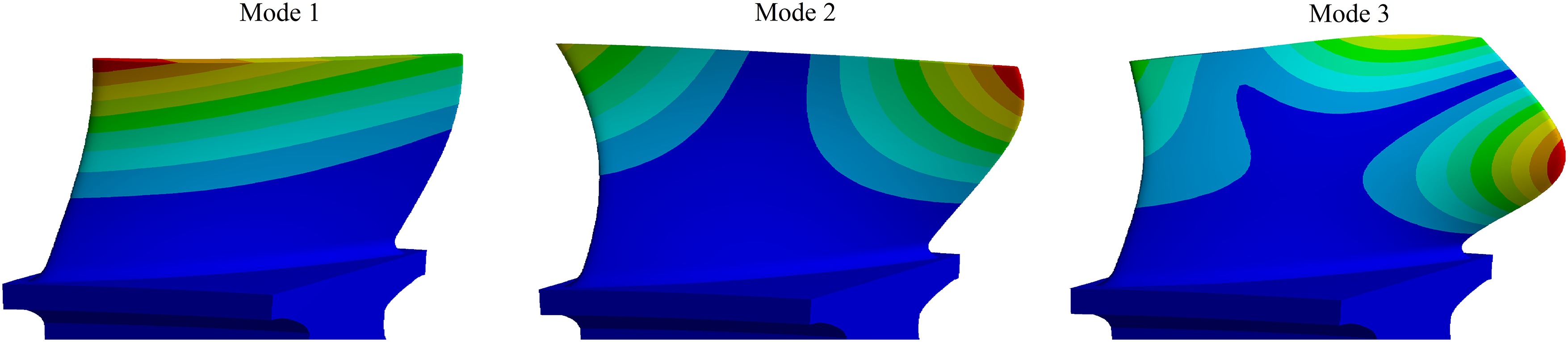
The finite elements method (FEM) solver ANSYS® (ANSYS Academic Research, Release 18.1) has been used for the structural analyses. After preliminary studies comparing different finite elements families, high-order tetrahedra have been chosen in place of hexaedra, pyramids or wedges. Although hexaedra could facilitate the mapping between solid and fluid grids, tetrahedra elements have proven to better model the current physics of the problem, particularly because regions with high stress gradients are better meshed. Similarly to the fluid domain, a grid independence study was performed for the solid meshes, this time with the first natural frequencies as comparative parameters. The grid convergence for two modes is displayed in Figure 5.
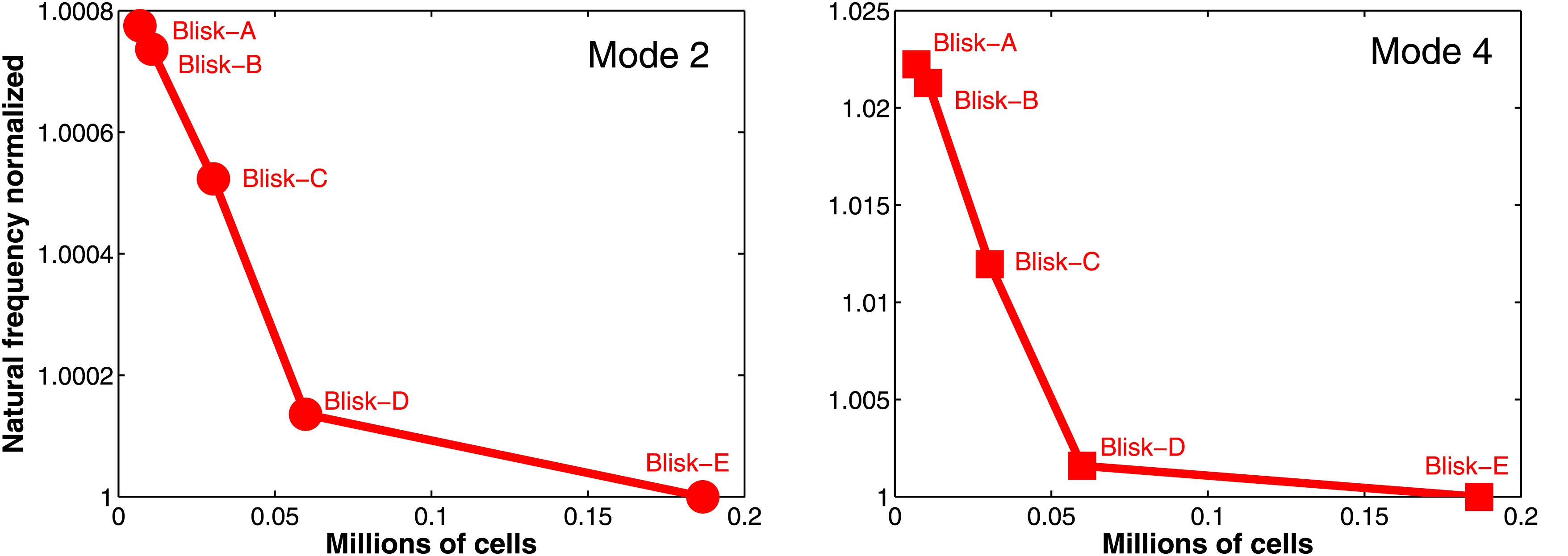
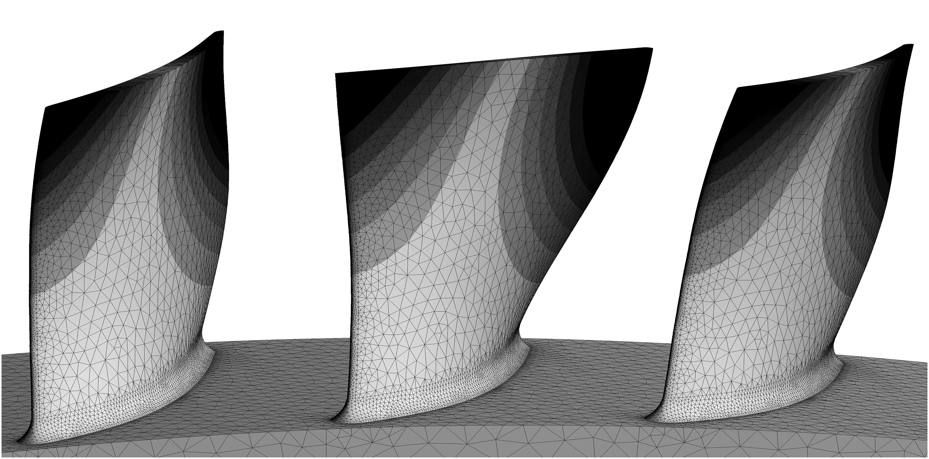
Even the coarsest of the generated meshes represents remarkably good the displayed modes (very similar behavior takes place for the first 20 mode shapes). However, the last but one finest mesh (labeled as Blisk-D) has been chosen to guarantee a good mapping between fluid and solid system variables. Each blade sector has 96322 nodes. This grid, expanded to cover the whole blisk, is shown in Figure 6, contoured with the second blade natural mode displacement, with 40 nodal diameters.
Figure 6.
Grid Blisk-D for the simulated rotor, obtained after grid independence study. Whole-circle expanded result displays the second blade natural mode (torsion) contours. Geometry is rescaled.
For brevity purposes, only a brief remark is made about the use of cyclic symmetry. In order to prevent the expensive modeling of the whole blisk structure, just one sector is meshed. Fourier decomposed boundary conditions are implemented on the symmetrical faces in the circumferential direction, with proper consideration of the total number of sectors (Thomas, 1979; Balasubramanian et al., 1991).
(ii) Harmonic forced response: subsequently to the prestressed modal analyses, mode-superposition harmonic response is computed. The time and frequency domain relations are displayed in Equation (4).
Here, as in classic FEM, M, C and K are the mass, damping and stiffness matrices, plus the displacement and forcing vectors U and F. Note that, since the forcing vector F(t) is complex when expanded into a harmonic series, real and imaginary aerodynamic forcing components must be inputted. Equation (4) shows the nodal coordinate
In the mode-superposition harmonic analyses, the first 117 natural modes have been used. A phase sweep was done, according to the studied target-frequency. The highest natural frequency obtained in the modal analysis setup was always at least 1.5 times the excitation frequency.
Results
Computational fluid dynamics
In this subsection, the CFD-only results are presented. Initially, time-domain calculations are assessed, showing how the disturbances affect performance, as well as the unsteady damping. Next, the frequency-domain results for aerodynamic damping are given.
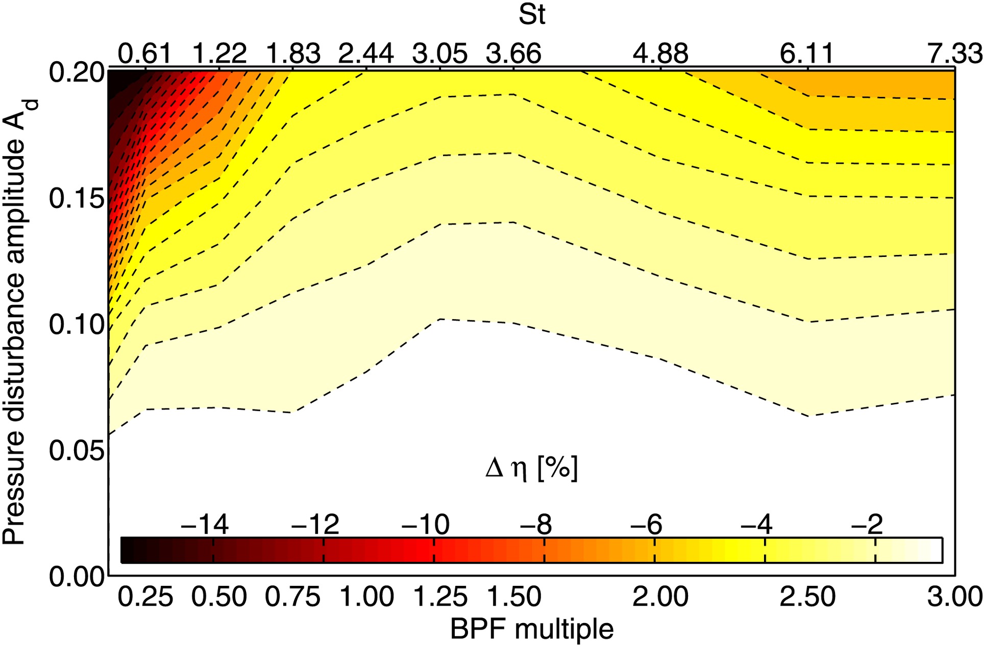
(i) Performance drop: the isentropic efficiency of the simulated stage was calculated for several disturbances patterns. Outlet static pressure amplitude and frequency have been varied according to current (and foreseen) PGC ranges. The amplitude
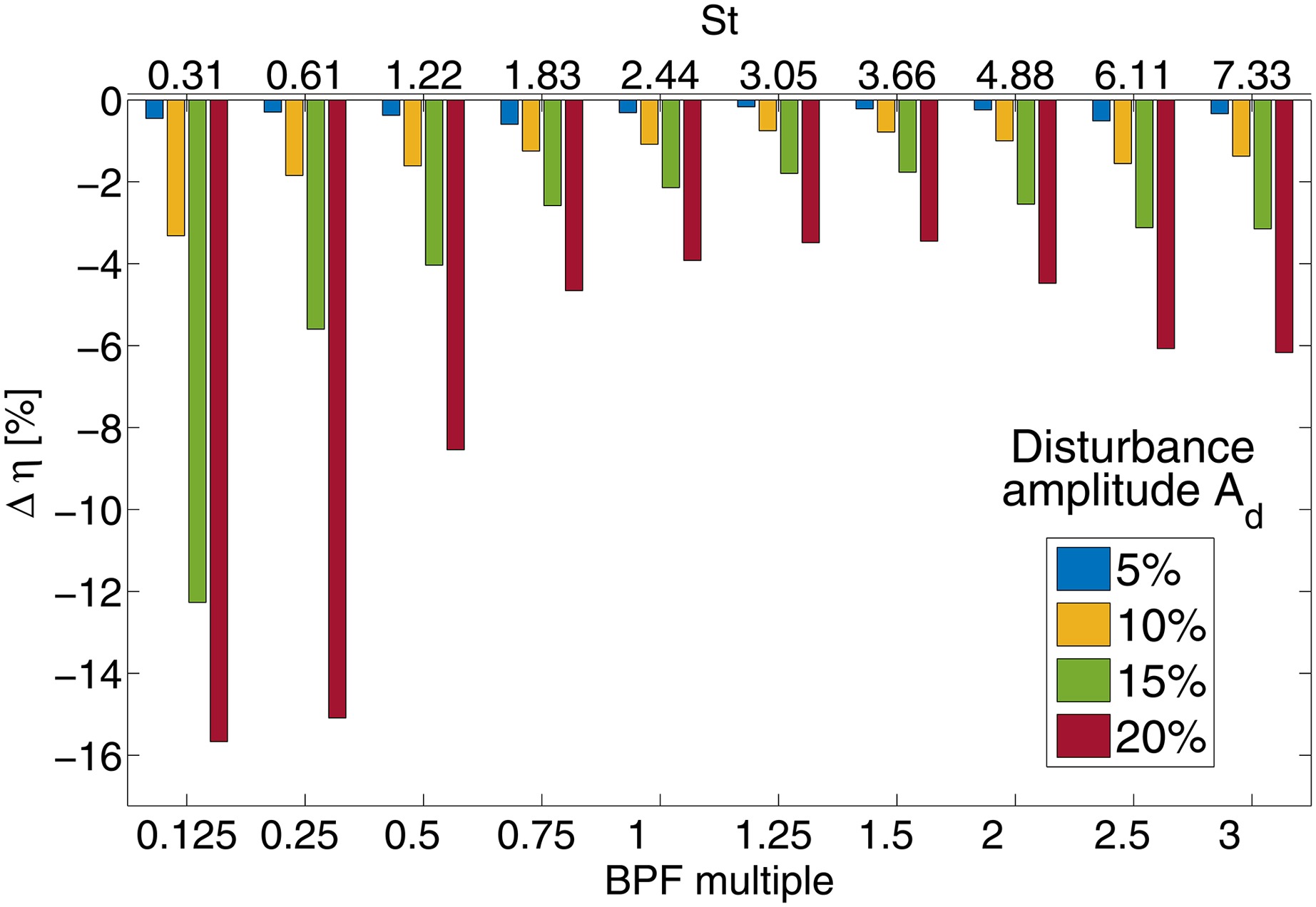
As a first trend, higher disturbance amplitudes
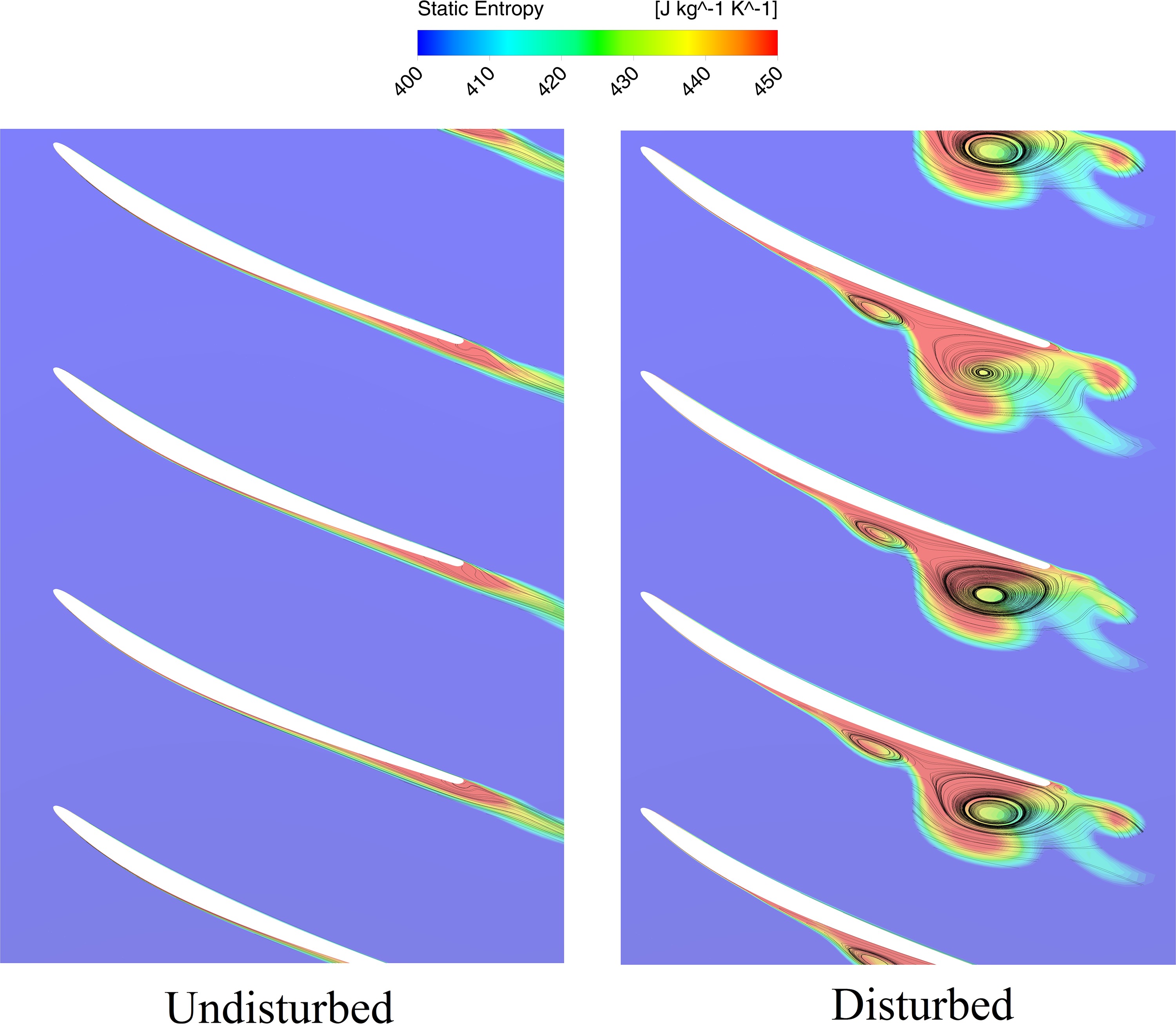
Figure 9.
Static entropy contour and surface streamlines around the rotor blade (cross section), for undisturbed and disturbed cases, with disturbance frequency of 0.25 BPF and amplitude 20%. A substantial increase in entropy and recirculation zones is present in the disturbed run. Geometry is rescaled.
(ii) Unsteady damping
The essence of the unsteady damping is to determine how much a state property unsteady variation is reduced
Figure 10.
Unsteady damping for disturbance amplitude of 20%. Pressure and temperature (static and total) values shown for several frequencies.
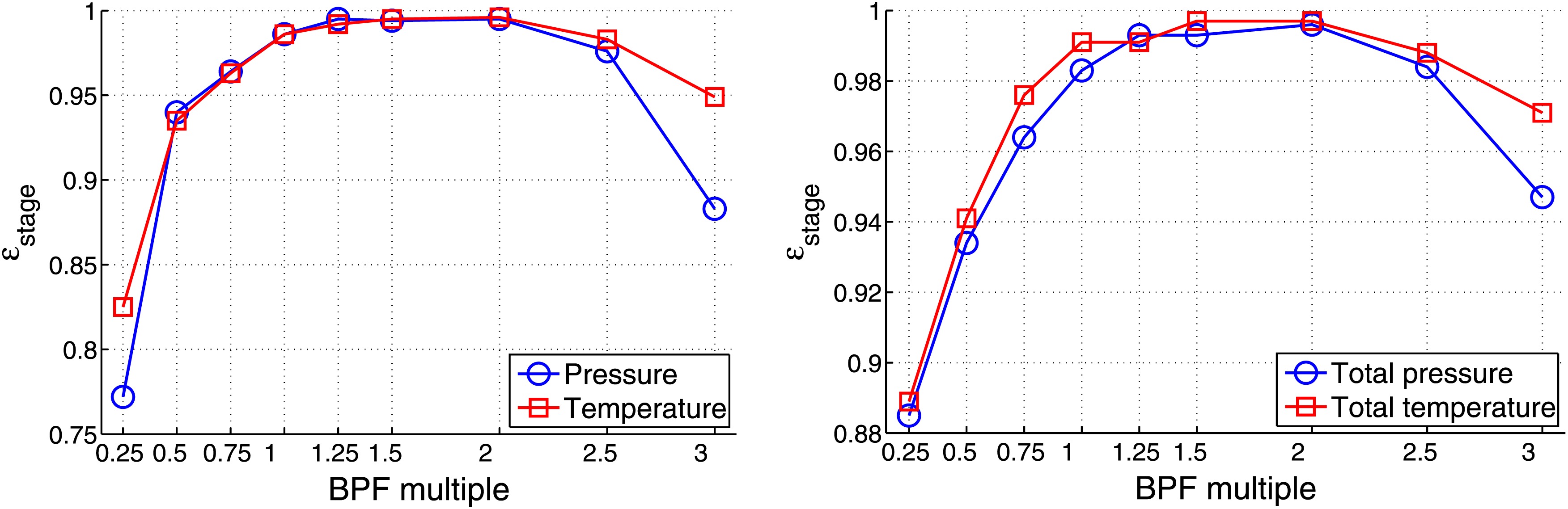
All unsteady damping values obtained are positive and close to 1 (that is, almost complete attenuation). Static and total unsteady damping show very similar behavior. However, very low and very high frequencies are less damped than the ones close to the BPF, when the disturbance propagates farther upstream. This is a valuable information for the aeroelasticity designer, since the blade structure should avoid (or at least withstand) vibrations at the adjacent excitation frequencies. The unsteady damping pinpoints how far the unsteadiness propagates along the streamwise direction, with high values (say, more than 95%) indicating that these fluctuations are weak enough when reaching the next stage, and therefore do not necessarily prompt redesign considerations.
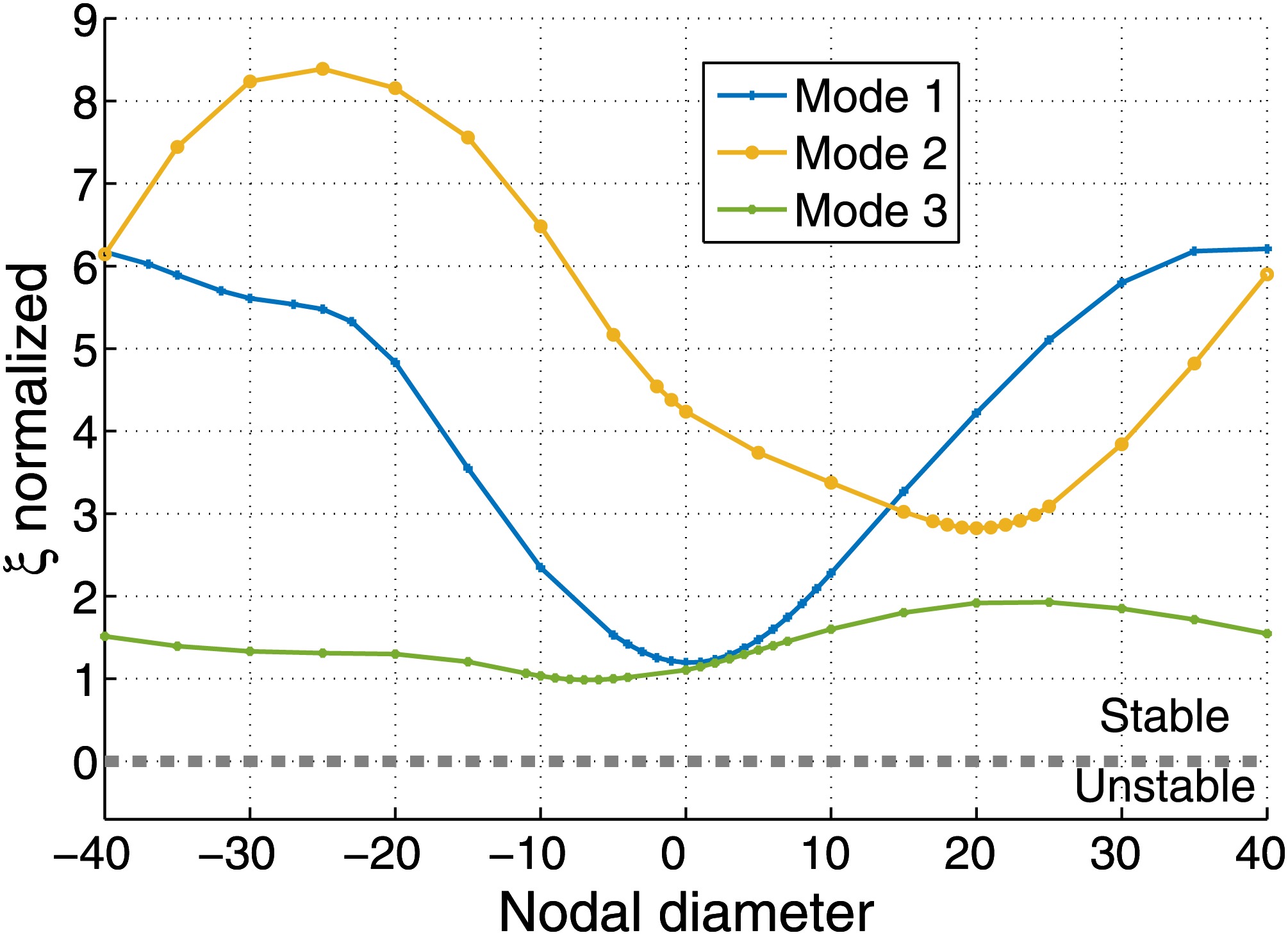
(iii) Aerodynamic damping: the aerodynamic work was used to determine the damping ratio
Subsequently, the damping ratio was calculated from the aerodynamic work, shown in Figure 13. Firstly, all simulated modes were shown to be stable for all nodal diameters (that is,
Computational solid mechanics
After the prestressed modal analysis, the next step is to identify the frequencies and forcing shapes which excite the structure. For these loads, the Campbell and interference diagrams, respectively, are convenient. Due to the exploratory character of this study, several cases have been run, however restricted to the nominal rotational speed of the machine.
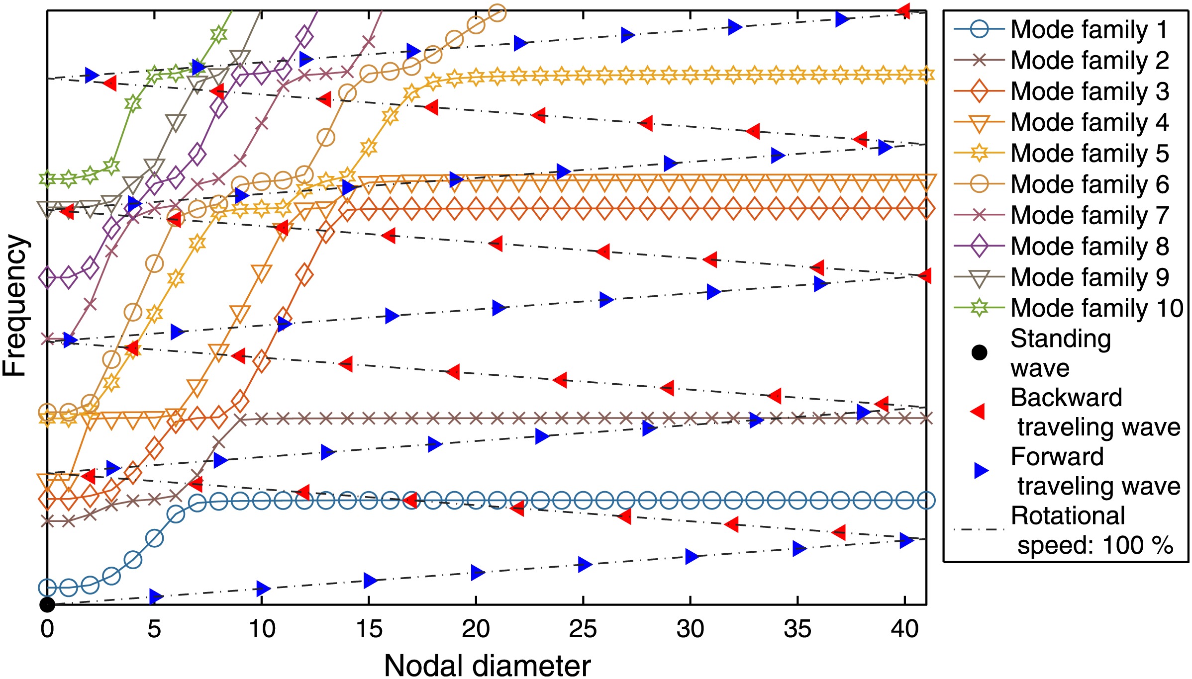
Along this manuscript, focus is cast on the disturbances originated from the combustor, although the stator perturbation (as seen by the rotor) is also naturally calculated. On that account, a sample interference diagram is shown in Figure 14, with five circumferentially scattered disturbance units downstream of the stage (which could correspond to detonation tubes, rotating-detonation chambers etc.). The inclination of the rotational speed line is determined not only by how fast the shaft spins, but also by the number of disturbance units. Therefore, for each choice of combustor units downstream, a new interference diagram is produced. The integral crossings between the speedline and the natural frequencies indicate which nodal diameter shapes are expected to be excited (Wildheim, 1979; Bertini et al., 2014).
Figure 14.
Sample interference diagram for simulated blisk, with the first ten mode shape families. An illustrative rotational speed line is indicated, for clear visibility purposes.
The simulated engine orders are directly correlated with the excitation frequency
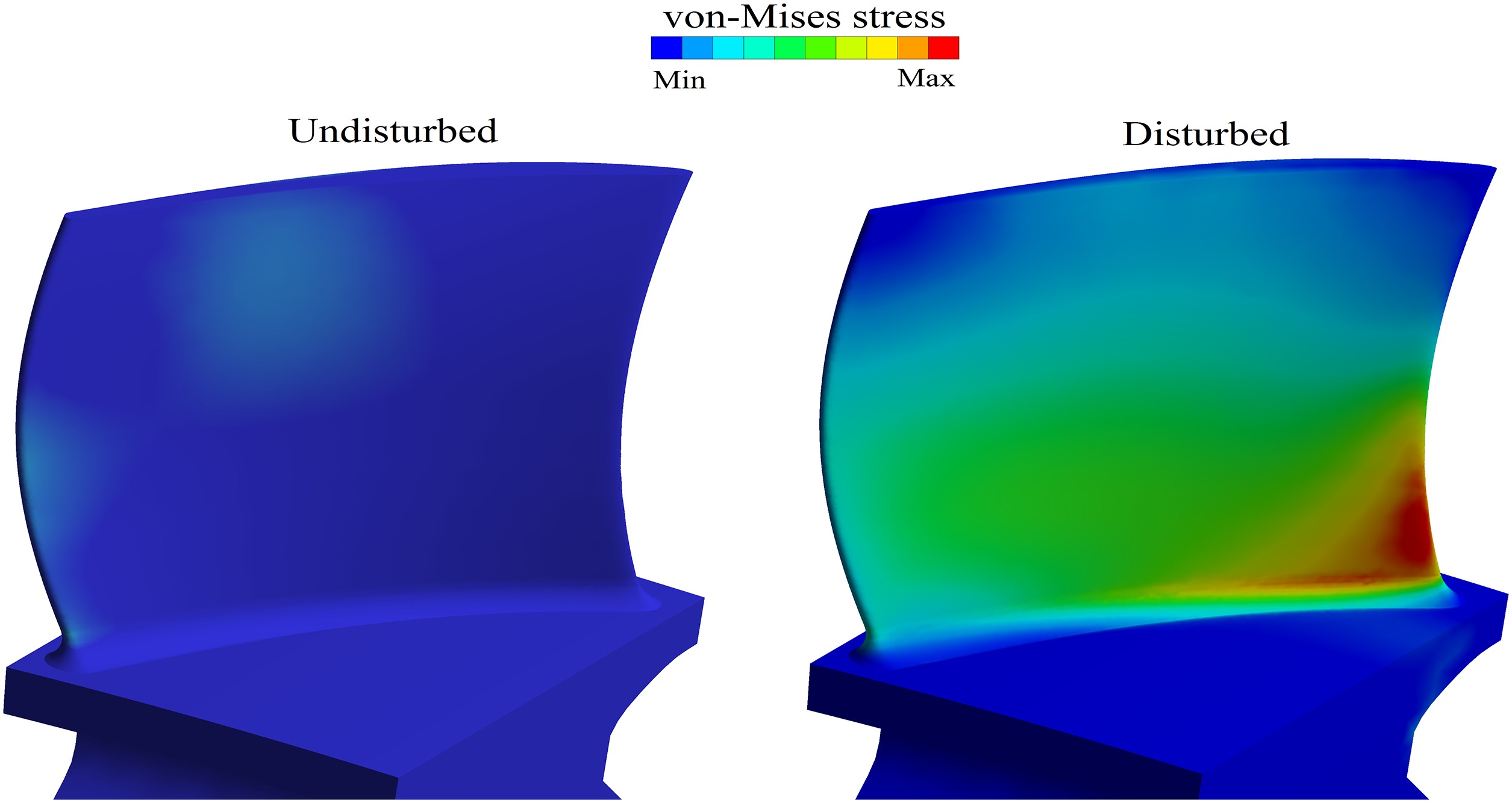
Figure 15 shows the maximum von-Mises stresses on the rotor blade for the undisturbed and the disturbed case, for
Figure 15.
Normalized von-Mises stresses on rotor blade for undisturbed and disturbed cases. The disturbance frequency is 0.125 BPF with amplitude 20%. Geometry is rescaled.
The maximum von-Mises stress on the rotor blisk is shown in Figures 16 and 17, for the disturbed computations. The normalization was done in two different ways. In Figure 16, all stresses were divided by the stress obtained in the 1.0 BPF disturbed run (any other value could be arbitrarily chosen, which would change only the vertical axis scale). The observed behavior matches qualitatively with the drop in efficiency, as well as the unsteady damping plots (depicted respectively in Figures 7 and 10). The stronger disturbance propagation observed in the low-frequency range excites the rotor blade more than the higher frequencies. Therefore, larger displacements and stresses are expected.
Figure 17.
Maximum von-Mises stresses on rotor blade for disturbed runs. Values normalized by the undisturbed results for each respective frequency.
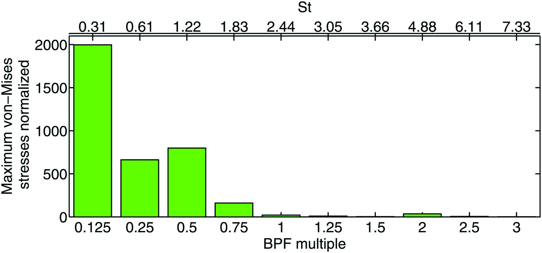
Figure 16.
Maximum von-Mises stresses on rotor blade for disturbed runs. Values normalized by the 1.0 BPF disturbance frequency results.
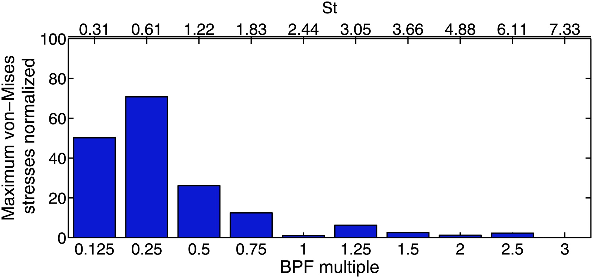
With respect to Figure 17, the normalization is accomplished dividing the maximum von-Mises stresses by the corresponding values obtained in the counterpart undisturbed runs. This is done independently for each excitation frequency. Low disturbance frequencies, again, promote higher stresses on the blade. The high values are expected, considering that, for the baseline undisturbed case, the strain induced on the blade due to the specified excitation frequencies is indeed minimal (except if specifically adjacent to BPF’s or eventual system fluctuations, such as rotating instabilities, are present). On the other hand, for the disturbed runs, the Fourier decomposition of the pressure will invariably yield much higher values close to the exciting frequencies. In spite of large relative values, the dynamic stress still remains under acceptable material limits (at least for the disturbance amplitudes here considered).
Conclusions
Numerical aeroelastic and high-accuracy CFD analyses were presented in this work, contrasting undisturbed and pressure gain disturbed operation of a typical industrial high pressure compressor stage. Due to the exploratory nature of this study, a wide range of disturbance frequencies and amplitudes was considered. The principal outcomes are:
From the turbomachinery component performance viewpoint, decrease in stage isentropic efficiency
The pressure and temperature unsteady damping (as defined in Equation (5)) was higher than 95%, for disturbance frequencies between 0.75 and 2.5 multiples of the BPF. Lower frequencies are particularly less unsteadily damped, meaning that the propagating disturbance should be perceptible to a greater extent upstream of the simulated stage.
The aerodynamic damping calculations exhibited no unstable nodal diameter for the operating point. The first three modes simulated with the nonlinear harmonic balance method displayed a fairly sinusoidal-like smooth behavior along the interblade phase angle spectrum. The global damping ratio
After a prestressed modal run, the rotor blisk was excited with the unsteady Fourier transformed forces, on mode-superposition harmonic response analyses. The horizontal comparison between different excitation frequencies followed the same behavior of the efficiency drop and unsteady damping. That is, the upstream propagating disturbances excite the rotor blade substantially more on the low-frequency end. Additionally, the von-Mises stresses obtained with the disturbed runs, anew for the lower frequencies, were several hundred times higher than the corresponding stresses for the undisturbed cases. For excitation frequencies higher than 1 BPF, this stress magnification is much more modest. Nonetheless, the stresses in all cases were still below material limits.
Nomenclature
disturbance amplitude
C
damping matrix
c
reference chord
complex modal coordinate
overdot for time derivative
complex modal forcing
disturbance frequency
K
stiffness matrix
surface integration coordinate
M
mass matrix
normal versor
pressure
scaling factor for FEM-CFD mapping
radius
St
Strouhal number
time
period
U
displacement vector
velocity vector
spatial coordinates vector
aerodynamic work
dimensionless wall distance