Introduction
Wall-bounded turbulent flows of organic fluids have drawn increasing attention in recent years, in part due to the application of organic Rankine cycle (ORC) systems for waste heat recovery. With wall-bounded flows present in the majority of ORC system components, an improved understanding of the detailed fluid mechanics within real-gas boundary layers is fundamental to (a) the validation of Computational Fluid Dynamics (CFD) codes, and therefore (b) the maximisation of component-level performance.
The majority of research within this area (Colonna et al., 2006; Colonna et al., 2008; Wheeler and Ong, 2014; Persico et al., 2015) has analysed blade-bounded flows in a turbine or nozzle, based upon the Reynolds Averaged Navier Stokes (RANS) simulation method. However further work is required for validation, to confirm that real-gas effects do not disturb the fundamental assumptions contained within RANS simulations.
Real-gas effects distinguish organic fluids from perfect gases such as air. The perfect-gas Equation of State (EoS), pV=RT, is inapplicable in these fluids when they work close to the saturation curve and/or critical point. In this case, the thermodynamic properties such as pressure, viscosity, and heat capacity, will depend not only on temperature, but also on density. As a result of this, many perfect-gas-based simplifications must be checked before their application. Meanwhile, most frequently-used organic fluids, including refrigerants, siloxanes and alkanes, have a large molecular weight and a high-level molecular complexity, also called dense gases (Cramer and Best, 1991; Kluwick, 2004).
Work by Colonna & Guardone (Colonna and Guardone, 2006) has shown that as the gas molecular complexity increases, its heat capacity, Cv/R, will increase, and the fundamental derivative of gas dynamics, Γ (defined in Equation 1 (Thompson, 1971)) will decrease. Perfect gases always have a constant Γ=(γ+1)/2 of more than unity, while dense gas can have a variable and lower Γ. For most of the frequently-used organic fluids, the minimum Γ can be lower than 1, where the speed of sound will decrease with pressure in an isentropic process (Thompson, 1971). There are also a group of theoretical BZT fluids (named after Bethe (Bethe, 1942), Zel’dovich (Zel’dovich et al., 1966) and Thompson (Thompson, 1971)), which contain a region of negative Γ. In that region an “inversion” of typical supersonic behaviour is observed, with flows achieving compression via fans, as opposed to shock waves (Thompson, 1971). To summarise, real-gas and dense-gas effects can have a significant influence on the mechanics of an organic fluid - it is the purpose of this work to study these effects in detail.
This work studies the real-gas effect on the turbulent boundary layer in a fully developed channel flow by means of Direct Numerical Simulation (DNS), in which no turbulence model is required due to flows being resolved down to the Kolmogorov microscale. DNS helps to get rid of the uncertainty caused by any turbulent modelling assumption, and produces the realization of a real-gas flow.
Kim, Moin & Moser (Kim et al., 1987) firstly applied the DNS method on a incompressible fully developed channel flow at Reynolds number of 3,300. They studied the turbulence statistics near the wall, and found that their results showed a good agreement with the experimental data.
Huang, Coleman & Bradshaw (Huang et al., 1995) studied compressible flow within a channel, and analysed the compressibility-associated terms in Reynolds averaged energy equations. They found that the averaged property profiles matched the corresponding incompressible curves well, by scaling by mean density, ρ¯/ρw. They also proposed the model for Reynolds analogy, mean-Favre-averaged fluctuations, and pressure-dilatation terms.
Patel et al (Patel et al., 2015) studied a turbulent channel with variable properties, in different cases of the relation between dynamic viscosity and temperature. They found that the normal Reynolds stress anisotropy and turbulence-to-mean time scales were influenced by that relation.
Sciacovelli, Cinnella, & Gloerfelt (Sciacovelli et al., 2017) studied a dense gas, PP11 (C14F24), in a turbulent channel flow. They focused on one operating point inside the region Γ<1, and found the mean temperature is nearly constant and the mean viscosity decreases from the wall to the centreline, showing a liquid-like behavior. Their results showed that dense gas channel flows can tend towards the behaviour of an incompressible channel flow with variable properties, due to their heat capacity.
The study within this work focuses on two commonly-used organic fluids, and compares three different working conditions of each fluid to give insight into the impact of real-gas effects. The main properties of these two organic fluids are show in Table 1. Refrigerant R1233zd(E), trans-1-chloro-3,3,3-trifluoropropene (CF3CH = CHCl), is accepted as a high-efficiency and environmental-friendly fluid for ORC systems, and it can be a substitute of refrigerant R245fa. Meanwhile, MDM, formally known as octamethyltrisiloxane (C8H24O2Si3), is a representative of the group of siloxane fluids, since they also can be a potential fluid of ORC systems.
Table 1.
| Property | R1233zd(E) | MDM |
|---|
| Tcr (K) | 439.6 | 564.1 |
| pcr (kPa) | 3,624 | 1,415 |
| ρcr (kg/m3) | 480.2 | 256.7 |
| M (kg/kmol) | 130.5 | 236.5 |
Methodology
Numerical method
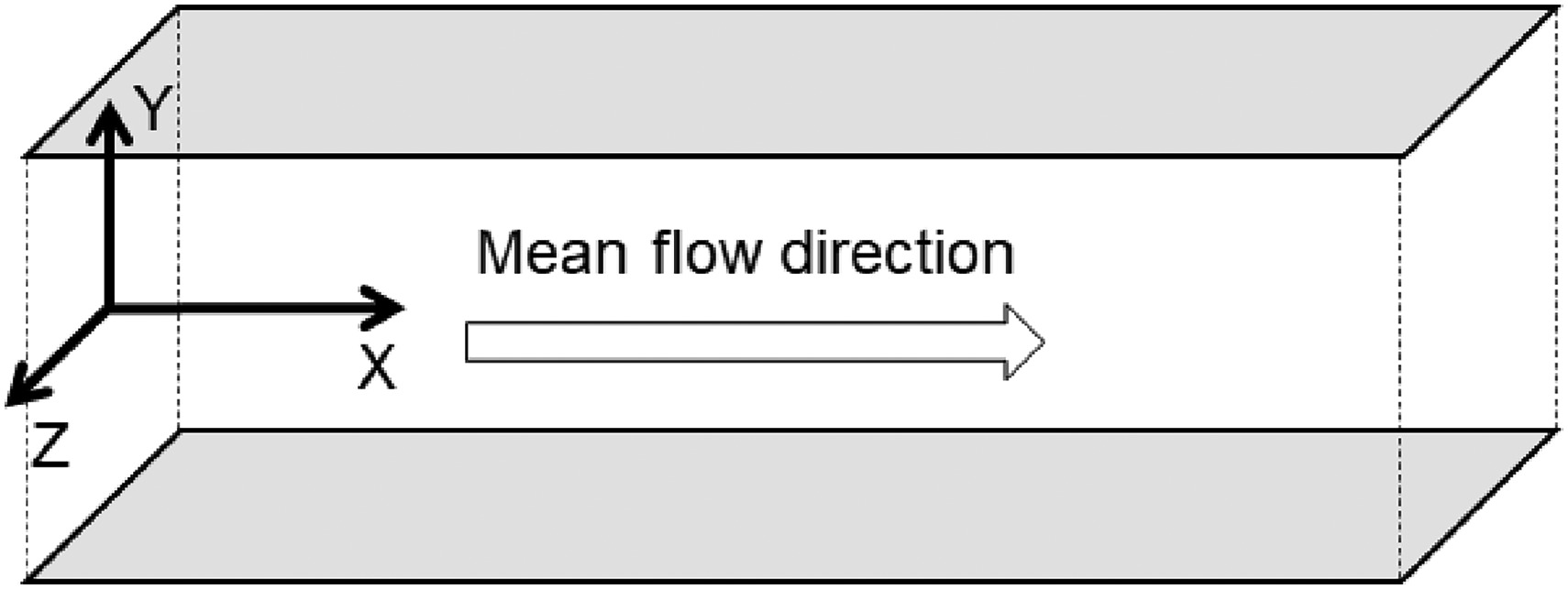
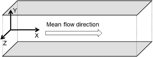
A fully developed channel flow is simulated in the domain shown in Figure 1, where the boundaries on X and Z direction are periodic boundaries and the boundary on Y direction is no-slip isothermal wall boundary - mean flow is in the X direction. The scale of the domain is Lx×Ly×Lz=2πh×2h×πh, where h is the characteristic length of the channel.
Figure 1.
Calculation domain of the channel flow simulation.
This work is based on the solution of the three-dimensional Navier-Stokes (NS) equations (Equations 2–4), which are closed by the equation of state p=p(ρ,T). These equations are non-dimensionalised by half-channel height, h, globally averaged density, ρG≡(1/h)∫0hρ¯dy, and global averaged velocity, uG≡(1/hρG)∫0hρu¯dy, before being calculated.
where:
Non-dimensional parameters can be declared as:
For a real gas, all the thermodynamic parameters are two-variable functions of both temperature and density. The global density and wall temperature (ρG, Tw) are taken to determinate the global dynamic viscosity, μG, and heat capacity Cp,G during the non-dimensionalisation. The global Reynolds number is defined by ReG≡(ρGuGh/μG) and the global Prandtl number is defined by PrG≡(Cp,GμG/λG). Subsequently, expression of the non-dimensional NS equations is the same as the original expression.
For the fully developed channel flow there is a periodic boundary instead of inlet and outlet boundaries, so the pressure drop along the stream is balanced by an artificial added body force fi, which is equivalent to the mean pressure gradient in physical flow (Huang et al., 1995). The body force fi is non-zero only for the mean flow direction (i=1), and it is uniform in the domain. The body force is calculated in each time step by keeping the global averaged mass flow rate invariant in the calculation.
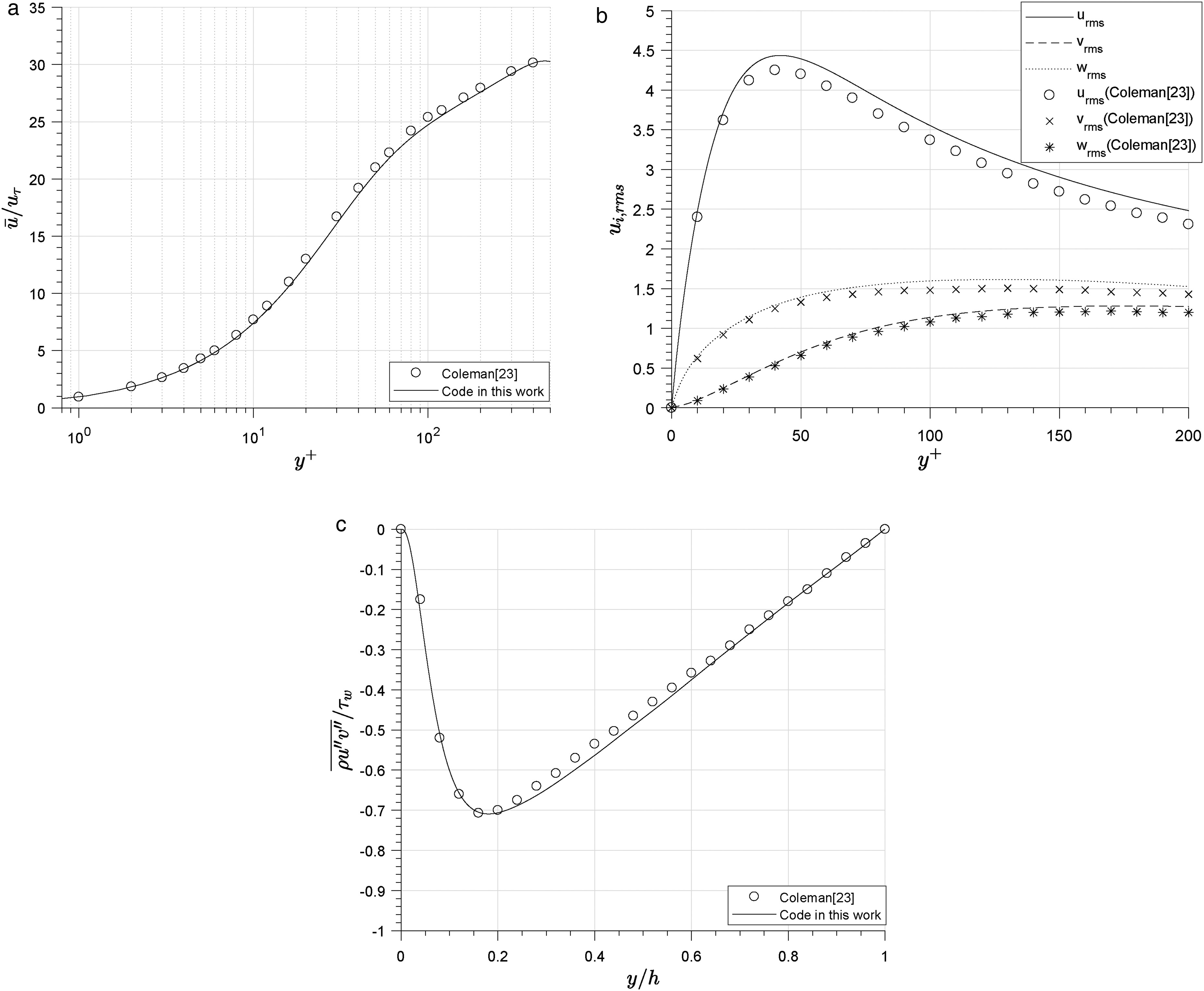
The DNS solver is developed based on a compressible DNS code from X. Li (Li et al., 2001) with an addition of a real-gas model. All the thermal properties in this model are two-variable functions of the local density and temperature, and they are calculated by the state-of-art Helmholtz energy EoS in REFPROP (Lemmon et al., 2007). Organic fluid cases are calculated by this real-gas model while the air case is calculated by a perfect-gas model. The NS equations are solved after non-dimensionalisation. For spectral discretisation, the convective flux derivatives are calculated by seventh-order upwind finite-difference scheme, and the viscous flux derivatives are calculated by sixth-order central scheme. For time advancement, it is solved by a third-order Runge-Kutta method. The validation of the simulation method is shown in the appendix.
The number of nodes in this work is Nx×Ny×Nz=128×257×128, and the overall number of nodes is 4.2 × 10⁶. The spatial resolution is chosen as DNS requirements. Zonta (Zonta et al., 2012) advised that (Δx/η)max≈12, (Δy/η)max≈2 and (Δz/η)max≈6, while Lee (Lee et al., 2013) advised that (Δx/η)max≈12.4, (Δy/η)max≈3.0 and (Δz/η)max≈7.9, where η is the smallest length scale in the flow. η is equal to the Kolmogorov length scale ηk when Prandtl number is lower than 1, while it equal to ηθ≈ηk/Pr when Prandtl number is higher than 1 (Monin et al., 1975). The spatial resolution of cases in this work is shown in Table 2, and it can fulfill the DNS requirement. The y+ of the first layer from wall boundary is below 0.5, and the first 10 layers are within y+=5.
Table 2.
DNS cases spatial resolution.
| Case | Air | R1 | R2 | R3 | M1 | M2 | M3 |
|---|
| (Δx/η)max | 12.6 | 9.9 | 11.1 | 14.3 | 9.4 | 9.4 | 10.6 |
| (Δy/η)max | 0.8 | 1.0 | 1.1 | 1.9 | 1.1 | 1.1 | 1.3 |
| (Δz/η)max | 6.3 | 5.0 | 5.6 | 7.1 | 4.7 | 4.7 | 5.3 |
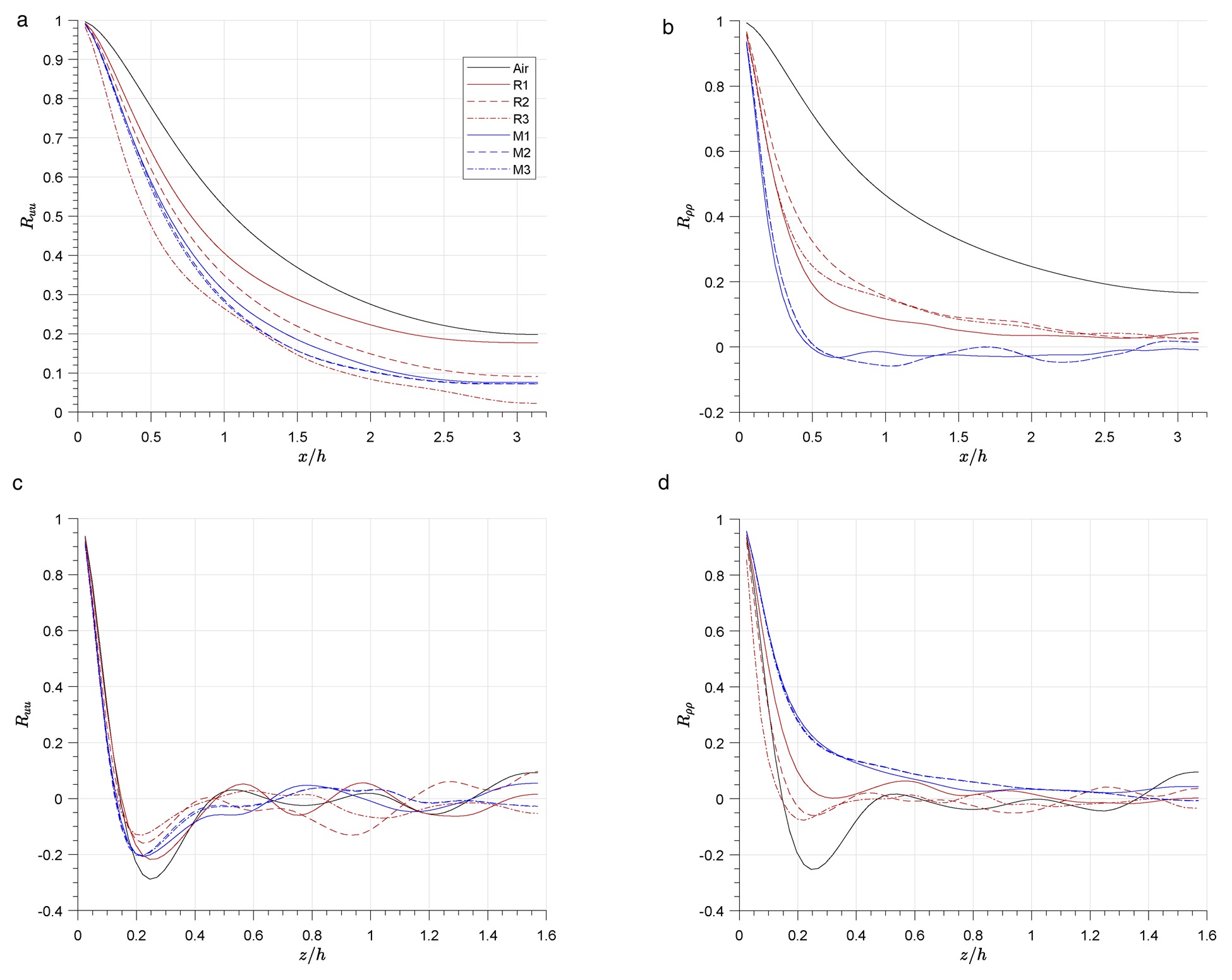
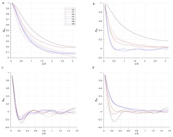
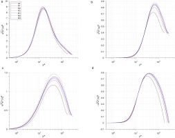
Figure 2a and 2b show two-point correlation of velocity u and density ρ between points in distance Δx∈[0,Lx/2] at y+≈10, and Figure 2c and 2d show the two-point correlation between points in distance Δz∈[0,Lz/2]. It shows that all the two-point correlations are close to zero at Lx/2 and Lz/2, which means that the domain size Lx and Lz are large enough for the channel flow cases with periodic boundary.
Figure 2.
Two-point correlation of velocity u and density in streamwise and spanwise. correlation in streamwise (a) and (b); correlation in spanwise (c) and (d).
This work is solved by the High Performance Computer in Imperial College London. Each case uses 512 CPUs, and it takes 10–20 days to get converged. After that, the statistic is taken every Δt^=2 within a time range Δt^=1000.
Case set-up
There are no standard inlet and outlet boundaries in this domain for the periodic boundary condition, so the global averaged density ρG and mass flow rate m˙G=uGhρG are set as an alternative. The global averaged velocity is given as uG=MaGcG, where MaG is the global Mach number. cG is a reference global sound speed defined by wall temperature and global averaged density cG=crg(ρG,Tw) for organic fluids, and only wall temperature cG=cpg(Tw) for air. The dynamic viscosity μG is defined in the same fashion - μG=μrg(ρG,Tw) for organic fluids and μG=μpg(Tw) for air. μrg is calculated by the real-gas model, and μpg is calculated by the Sutherland viscosity law (Sutherland, 1893) shown in Equation 16, where Ts = 110.56 K is the effective temperature.
The initial condition is a turbulent flow field, in which the global averaged density ρG and mass flow rate m˙G are set. During the calculating, ρG and m˙G will not change. After each time step, ρG is calculated and compared with its value in the previous step. If there is a gap between them (caused by numerical error), the density at all points will plus or minus a same small density source term Δρ so as to keep ρG invariant after this step. m˙G is also calculated in each step and compared with its value in the previous step. If they are different, the body force will be changed so as to maintain an invariant m˙G.
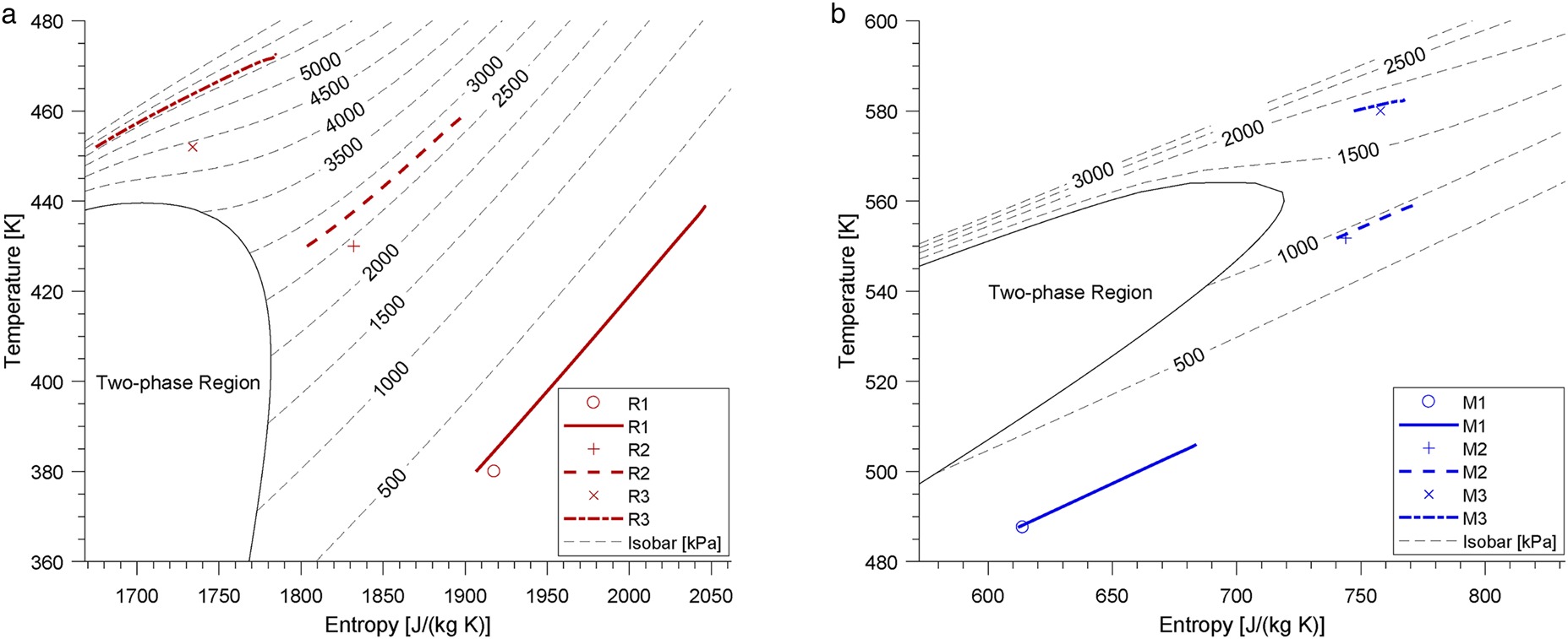
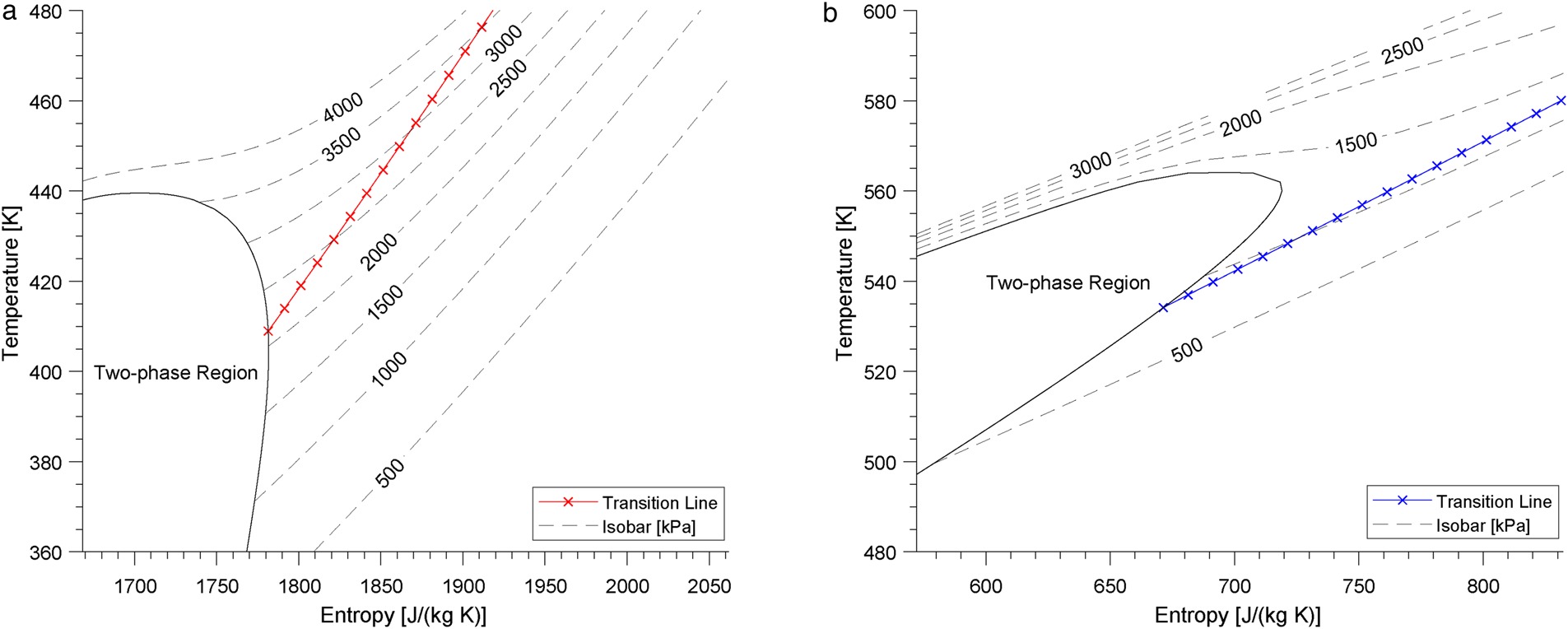
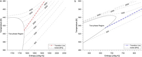
The global Mach number MaG≡(uG/cG) and global Reynolds number ReG≡(ρGuGh/μG) are set at 2.25 and 4,880 for all seven cases. The air case follows the perfect-gas Equation of State, requiring only one thermodynamic condition - the wall temperature, Tw = 288 K. The two thermodynamic conditions chosen for the real-gas cases were wall temperature and global density. From R1 to R3, the set-up point moves closer to the supercritical region, shown by the temperature-entropy diagram in Figure 3. The red and blue lines in Figure 3 are the averaged thermodynamic property distribution in each real-gas case. Cv/R for each case is list in Table 3, and the value for MDM is the largest whilst air is the smallest. As the set-up point closer to the supercritical region Cv/R increases, although this change is small in comparison to the difference in values between R1233zd(E) and MDM. The fundamental derivative Γ shows that the minimum value is at R2 and M2 for the two organic fluids, respectively.
Figure 3.
Temperature-entropy diagram of R1233zd(E) and MDM. Dots refer to set-up cases, whilst lines refer to mean thermal property distribution. (a) R1233zd(E) (b) MDM.
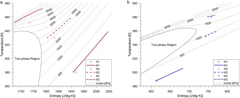
Table 3.
Calculating conditions for case set-up (R = R1233zd(E), M = MDM).
| Case | Air | R1 | R2 | R3 | M1 | M2 | M3 |
|---|
| Tw/Tcr | — | 0.86 | 0.98 | 1.03 | 0.86 | 0.98 | 1.03 |
| ρG/ρcr | — | 0.02 | 0.27 | 1.00 | 0.02 | 0.27 | 1.00 |
| ReG | 4,880 | 4,880 | 4,880 | 4,880 | 4,880 | 4,880 | 4,880 |
| MaG | 2.25 | 2.25 | 2.25 | 2.25 | 2.25 | 2.25 | 2.25 |
| Cν,G/R | 2.5 | 13.4 | 15.7 | 17.3 | 53.1 | 58.3 | 61.9 |
| Γ | 1.2 | 1.01 | 0.82 | 1.90 | 0.97 | 0.59 | 1.62 |
| Z | 1 | 0.96 | 0.67 | 0.32 | 0.96 | 0.68 | 0.33 |
Results and discussion
Averaged velocity and thermodynamic properties
The variables are averaged on each y level, since the x and z directions are periodic. For analysis, the wall shear stress is defined as the averaged value τw≡[μ(∂u/∂y)]¯w and wall friction velocity is defined as uτ≡τw/ρ¯w. Huang et al (Huang et al., 1995) proposed a semi-local friction velocity uτ∗≡τw/ρ¯ as well, which takes compressibility effects into consideration.
Some important global results of each case are listed in Table 4. Bulk Reynolds number and bulk Mach number are defined as ReB≡ρGuGh/μ¯w and MaB≡uG/c¯w (Sciacovelli et al., 2017), and they are different from ReG and MaG in real gases (μ¯w≠μG).
Table 4.
DNS results for each case.
| Case | Air | R1 | R2 | R3 | M1 | M2 | M3 |
|---|
| ReB | 4,880.0 | 4,881.1 | 4,530.4 | 2,683.1 | 4,880.7 | 4,836.4 | 4,175.0 |
| ReC | 3,512.5 | 4,824.6 | 5,219.2 | 5,648.0 | 5,394.9 | 5,519.9 | 5,632.4 |
| MaB | 2.25 | 2.26 | 2.52 | 1.26 | 2.25 | 2.32 | 2.09 |
| MaC | 1.92 | 2.40 | 2.34 | 2.21 | 2.53 | 2.50 | 2.51 |
| Reτ,C | 395.9 | 306.9 | 306.2 | 205.7 | 287.6 | 287.9 | 262.9 |
| Reτ,C∗ | 183.4 | 243.4 | 266.0 | 300.7 | 270.1 | 277.4 | 287.8 |
| T¯C/Tw | 1.875 | 1.155 | 1.069 | 1.045 | 1.038 | 1.014 | 1.004 |
| PrGEcG | 0.28 | 0.055 | 0.025 | 0.018 | 0.013 | 0.005 | 0.002 |
| PrG | 0.7 | 0.81 | 1.02 | 4.77 | 0.73 | 0.67 | 1.41 |
| EcG | 0.4 | 0.069 | 0.025 | 0.004 | 0.017 | 0.007 | 0.001 |
| Cp,G/R | 3.5 | 14.7 | 21.7 | 81.3 | 54.3 | 64.5 | 139.4 |
| ρ¯w/ρ¯c | 1.89 | 1.18 | 1.33 | 1.52 | 1.05 | 1.07 | 1.14 |
| −(∂ρ^/∂T^)p,G | 1 | 1.1 | 3.9 | 31.4 | 1.1 | 3.9 | 33.3 |
| p^w¯ | 0.26 | 0.22 | 0.28 | 0.27 | 0.21 | 0.31 | 0.43 |
| μ¯c/μ¯w | 1.57 | 1.16 | 1.00 | 0.56 | 1.04 | 1.01 | 0.86 |
The centre-line Reynolds number and Mach number are defined as ReC≡ρ¯Cu¯Ch/μ¯C and MaC≡uC/cC¯.The values show that ReB decreases as the set-up point is closer to the supercritical region (from R1 to R3 and from M1 to M3), while ReC increases. Both organic fluids have smaller ReB and larger ReC relative to the air baseline. The Mach number MaB firstly increases and then decreases as the set-up point is closer to the supercritical region (from R1 to R3 and from M1 to M3), while the centreline Mach number shows minimal change across cases.
The friction Reynolds number is defined as Reτ≡ρ¯wuτh/μ¯w. The friction Reynolds number is lower in the organic fluid cases than air, while lowest in the supercritical cases (R3 and M3). The semi-local friction Reynold number Reτ∗≡ρ¯uτ∗h/μ¯ has a higher value for the two organic gases than air, and Reτ∗ is highest in the supercritical cases R3 and M3 for each fluid.
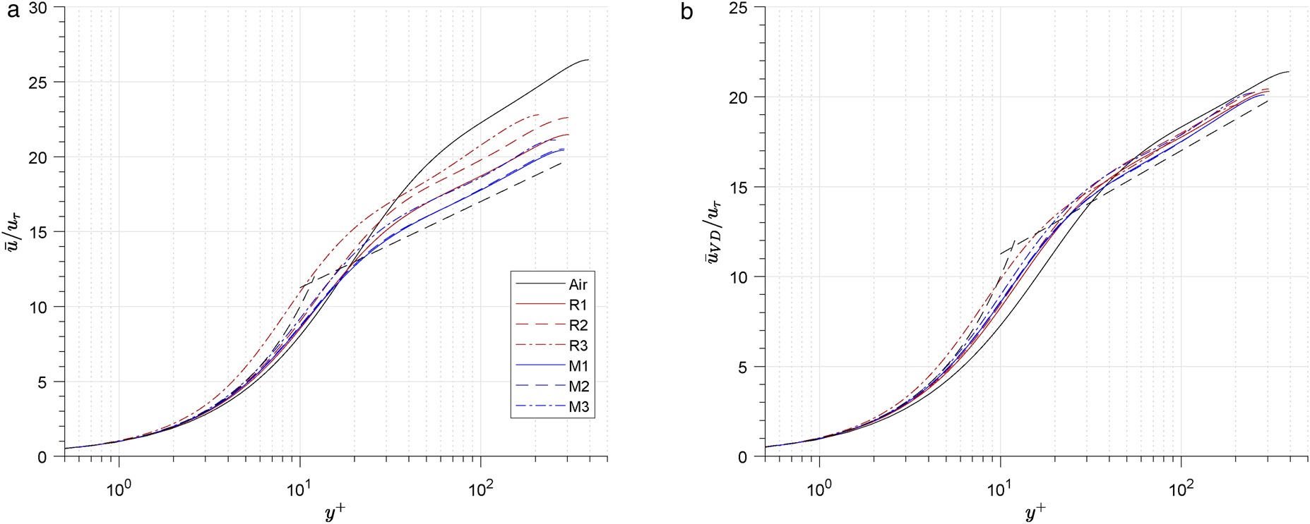
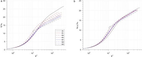
Reynolds averaged velocity and distribution versus non-dimensional wall distance y+≡ρ¯wuτy/μ¯w is shown in Figure 4a The position y+=0 is the wall, while the maximum y+ is the central layer of the channel. It shows that the organic fluid cases are closer to the log law line u+=0.25 ln (y+)+5.5 in the outer layer than air. In each fluid, as the case moves closer to the supercritical region, the velocity distribution increases in deviation from the log law line. After the application of a Van Driest transformation (Equation 17) (Van Driest, 1951) good agreement to the log law in the outer layer is observed (shown in Figure 4b).
Figure 4.
Distribution of x-direction averaged velocity along wall distance. black dashed lines refer to u+=y+ in the viscous sublayer and u+=0.25ln(y+)+5.5 in the outer layer.
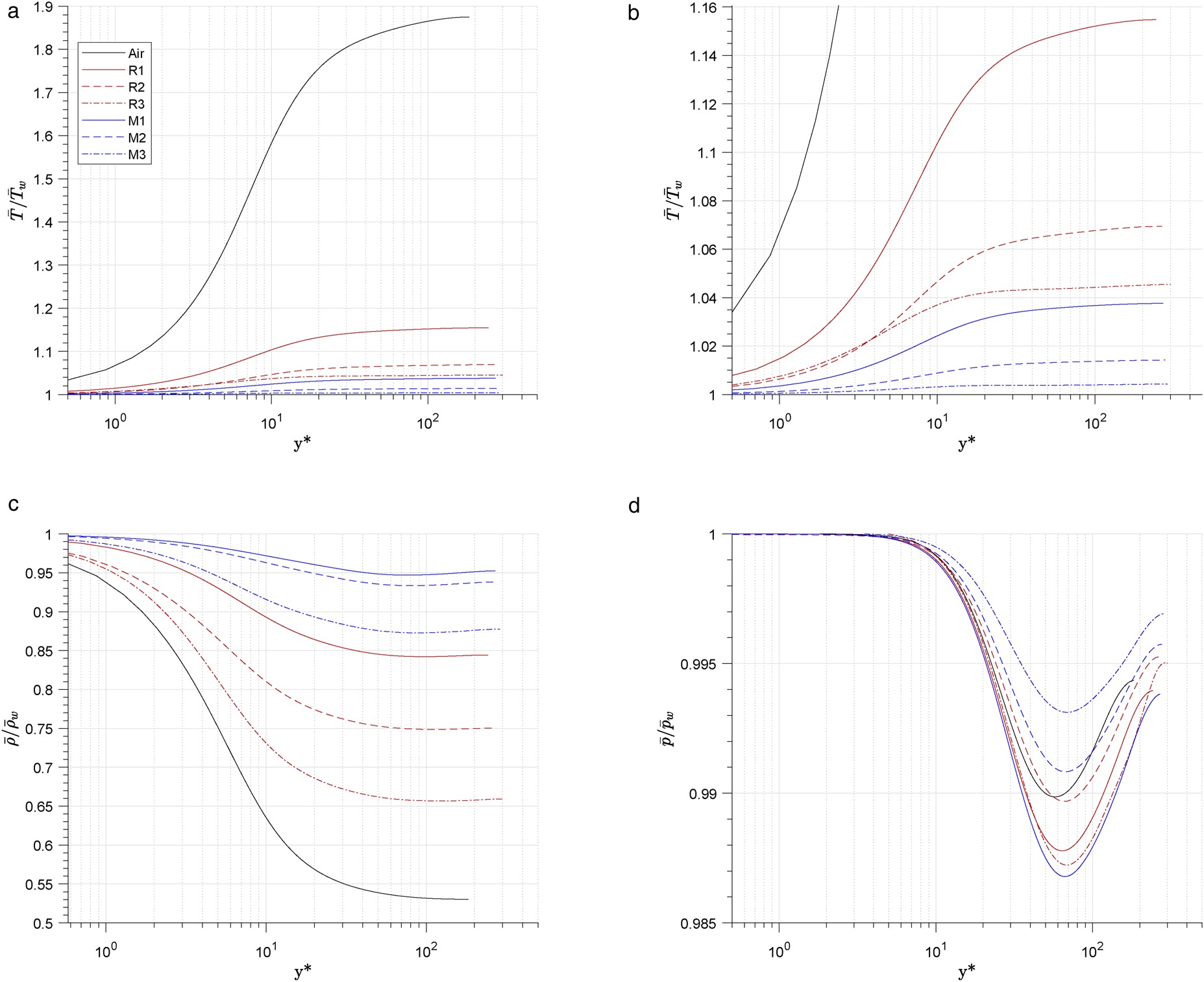
The averaged temperature, density and pressure along the wall-normal direction are shown in Figure 5, where the abscissa is the non-dimensional wall distance y∗≡ρ¯uτ∗y/μ¯. Figure 5a shows that the temperature in the central region of the channel is higher than wall temperature, and centre-to-wall temperature ratio T¯C/Tw is lower in the organic fluid cases than in the air case (shown in Table 4).
Figure 5.
Distribution of averaged temperature, density and pressure along the wall-normal direction. (a) Averaged temperature. (b) Averaged temperature (zoomed). (c) Averaged density. (d) Averaged pressure.
For each organic fluid, T¯C/Tw decreases as the point moves closer to the supercritical region (R1 to R3 and M1 to M3). T¯C/Tw correlated positively to PrEc in these cases (Prandtl number Pr≡Cpμ/λ, Eckert number Ec≡c2/CpT), which means the larger PrEc the larger T¯c/Tw will be.
When averaging and integrating the energy equation, the heat transfer as a function of wall distance can be represented by Equation 18 [12]. In the expression, Fu(y) is a velocity distribution function which equal to 0 at y^=0 and equal to 1 at y^=1. Since the heat conductivity fluctuation is small compared with averaged conductivity, the gradient of averaged temperature can be derived to Equation 19.
By assuming the velocity distribution function and the thermal conductivity ratio the same in all these cases, the non-dimensional temperature gradient is approximately proportional to the global Prandtl number multiplied by global Eckert number PrGEcG whose values are shown in Table 4. For a perfect gas, EcG=γR/Cp=γ−1. The organic fluids have higher molecular complexity, leading to a larger Cp/R and therefore a smaller Ec. For each organic fluid, Pr and Ec are variable, and the closer to the super critical region the smaller the value of PrEc.
The density is higher at the channel wall than the channel centre (shown in Figure 5c, and the value of the wall-to-centre density ratio ρ¯w/ρ¯C is shown in Table 4. The largest density ratio also appears in the air case, which is the same for the temperature ratio mentioned above. However, for each organic fluid, the density ratio increases as the set-up point moves closer to the supercritical region, while the temperature ratio has a reverse trend.
Since the pressure is nearly constant (p¯/p¯w>0.985 shown in Figure 5d), the density gradient is approximately equal to the temperature gradient multiplied by −(∂ρ^/∂T^)p (Equation 21). The value of −(∂ρ^/∂T^)p is shown in Table 4. It is equal to 1 in perfect gas, but it increases significantly as the set-up point moves closer to the supercritical region in real gases(from R1 to R3, and M1 to M3). The effect of the increase in −(∂ρ^/∂T^)p is larger than that of the decrease in temperature gradient, so the density drop is larger in cases closer to the supercritical region.
The pressure ratio has a minimum value at y∗≈70 for all the cases (shown in Figure 5d). As the set-up point moves closer to the supercritical region, the maximum pressure drop firstly increases and then decreases in R1233zd(E) (from R1 to R3), while it increases monotonically in MDM (from M1 to M3). This trend of maximum pressure drop is nearly negatively related to the averaged pressure at wall p^¯w (shown in Table 3), and this relation can be explained by the Reynolds averaged momentum equation in the y direction (Equation 22) in the following paragraph.
After integrating Equation 22 along wall distance y, the expression of for pressure ratio shown in Equation 23 is found. The pressure ratio is associated to 1/p^¯w and ∫0y(d(ρ¯v′′v′′~)/dy)dy. If the later part differs slightly between cases, it can be concluded that the larger the wall pressure p^¯w is the smaller the pressure drop will be.
The distribution of averaged dynamic viscosity ratio μ¯/μ¯w is shown in Figure 6. It shows that the viscosity increases as y∗ increases in the Air baseline, R1 and M1, while it decreases in Case R3 and M3. Sciacovelli et al (Sciacovelli et al., 2017) proposed that the former trend is a gas-like behaviour while the latter is a liquid-like behaviour, and that liquid-like behaviours can be observed in dense-gases.
Figure 6.
Distribution of averaged dynamic viscosity along the wall-normal direction.
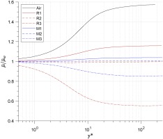
From the result of Figure 6, it shows that the liquid-like behaviour only exists in the supercritical cases (R3 and M3) of the two organic fluids. By implication there is a transition line from gas-like behaviour to liquid-like behaviour in each organic fluid, which is (∂μ/∂T)p=0 shown in Figure 7. The slope of the transition line is larger than that of the isobar lines. When fluid works below the transition line, the dynamic viscosity increases with wall distance; otherwise when fluid works above that line, the dynamic viscosity decreases as wall distance is increased.
Figure 7.
Transition line for R1233zd(E) and MDM. (a) R1233zd(E). (b) MDM.
Reynolds stress
The distributions of Reynolds stresses u′′u′′~, v′′v′′~, w′′w′′~ and u′′v′′~ normalized by uτ∗2 are shown in Figure 8. The normal Reynolds stress in the streamwise direction, u′′u′′~, shows a slight deviation (less than 4%) between cases (shown in Figure 8a), while the normal Reynolds stress in spanwise and wall-normal directions (v′′v′′~and w′′w′′~) show larger values of deviation (Figure 8b and 8c).
Figure 8.
Distribution of reynolds stresses.
The peak values of v′′v′′~ in real-gas cases are larger than that in air case by 7–20%. For each fluid, when the real-gas effect increases(from R1 to R3, or M1 to M3), the peak value will increase. Meanwhile, this impact is stronger in R1233zd(E) than in MDM. Real-gas effect also influence the peak values of w′′w′′~, which are larger by 10–21% in real-gas cases. The trend of this impact is the same as that of the real-gas effect on v′′v′′~.
The impact of real-gas effect on the normal Reynolds stress in spanwise and wall-normal directions (v′′v′′~ and w′′w′′~) is associated with the viscosity profile and bulk Reynolds number ReB. Patel et al. (Patel et al., 2015) proposed that if the centre-to-wall viscosity ratio less than 1, the normal Reynolds stress in spanwise and wall-normal directions will increase, and Sciacovelli et al (Sciacovelli et al., 2017) proposed that the increase of bulk Reynolds number ReB will lead to a larger peak value of normal Reynolds stress. Both these two effects influence the normal Reynolds stress in the cases of this work, while the viscosity ratio effect seems more predominant in this work, since supercritical case R3 (with the lowest μ¯c/μ¯w and lowest ReB) has the largest maximum v′′v′′~ and w′′w′′~ among all cases.
The Reynolds shear stress u′′v′′~ is larger in two organic fluids by (5–8%) in comparison to air, while the difference between organic fluid cases is not significant. The maximum value of Reynolds shear stress u′′v′′~ is associated with the viscous shear stress. According to the Reynolds averaged momentum equation in the y direction (Equation 24), the viscous shear stress and Reynolds shear stress balance the body force together. Since the dynamic viscosity for real-gas cases is smaller in the outer layer, which leads to a smaller viscous shear stress, so the Reynolds shear stress becomes larger compared with air case.
Turbulence energy
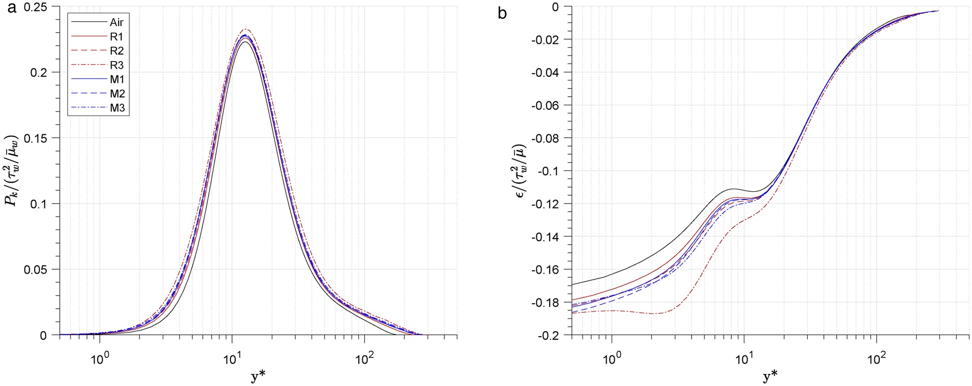
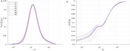
The Reynolds averaged turbulence energy equation for fully developed channel flow is shown in Equation 25. The first term is turbulence energy production Pk; the second term is the summary of turbulent diffusion, velocity-pressure diffusion, and viscous diffusion; the third term is energy dissipation ϵk; and the last three terms are compressibility-related terms. The turbulence energy production term Pk and dissipation term ϵk are discussed in this work, which are defined in Equations 26 and 27.
The distribution of turbulence energy production Pk is shown in Figure 9a. It shows that the fluid property do not significantly influence non-dimensional turbulence energy production, with a maximum Pk difference of less than 5% across all cases. The distribution of turbulence energy dissipation ϵk is shown in Figure 9b. The difference between the air and real-gas cases are significant in the viscous sublayer and buffer layer (y∗<30), with the magnitude decreasing in the outer layer (y∗>30). The non-dimensional dissipation at the wall is 5–13% higher in real-gas cases than air. For each organic case, the non-dimensional dissipation in the viscous sublayer and buffer layer increases as the real-gas effect increases (from R1 to R3; M1 to M3).
Figure 9.
Distribution of turbulence energy (a) Production, (b) Dissipation.
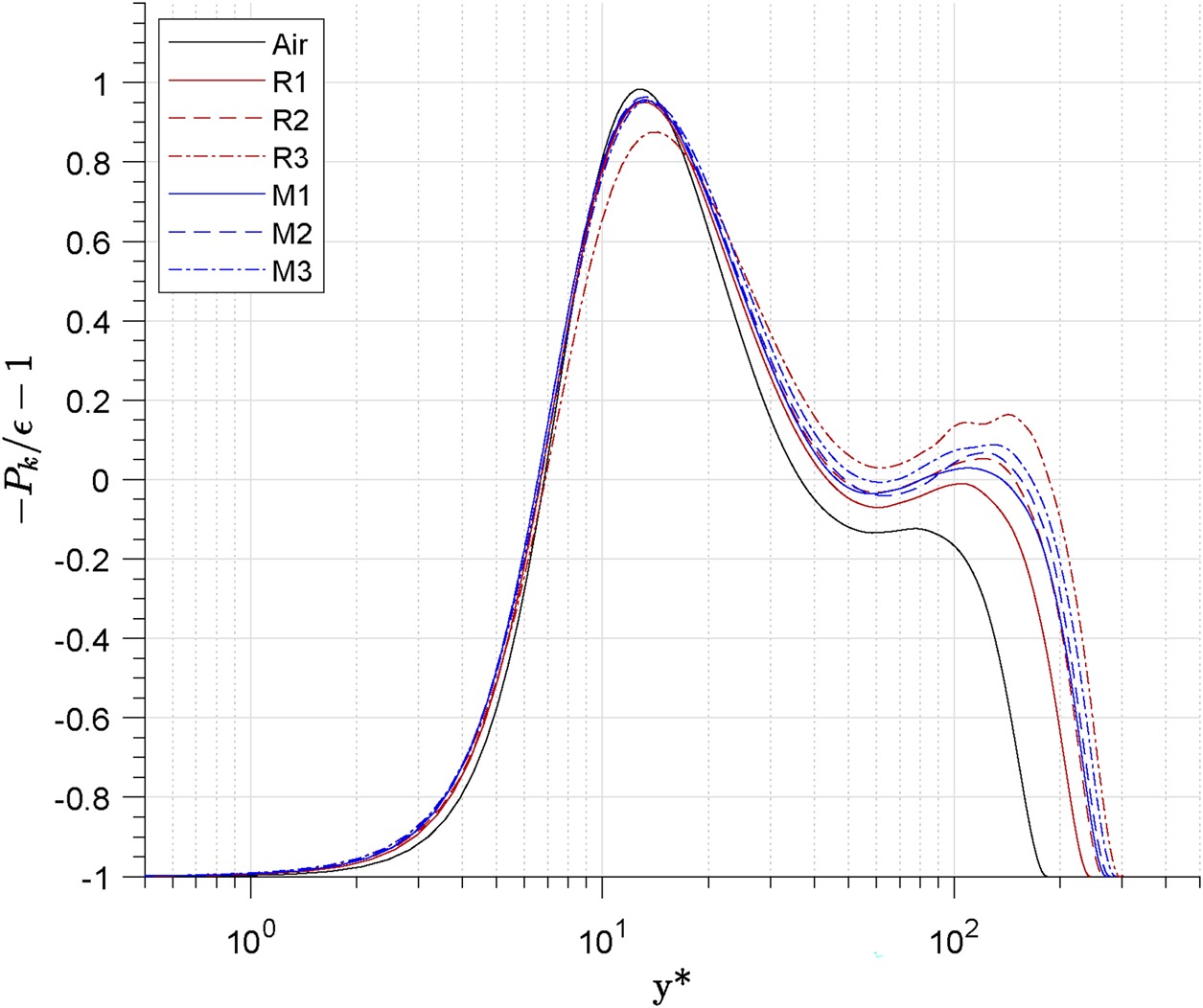
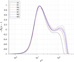
The turbulence energy production-to-dissipation ratio −Pk/ϵ−1 is shown in Figure 10. A clear peak is demonstrated at y∗≈10 across all cases, followed by a reduction to nearly zero as y∗≈50 is reached. In the region y∗>50, the air case remains stable before reducing to −1, while those for real-gas cases will increase slowly before demonstrating the same decrease (albeit at higher values of y∗). The position of the start point for the second drop is related to Reτ,C∗, and the larger the Reτ,C∗ the later the second drop will be.
Figure 10.
Distribution of turbulence energy production - to - dissipation ratio.
Turbulence viscosity hypothesis
The evaluation of the turbulence viscosity hypothesis for the standard two-function RANS model (k−ϵ and k−ω) is a focus of study in this work. The turbulence viscosity νt is defined as the ratio of Reynolds shear stress to the gradient of the averaged velocity, whose simplified expression in the full developed channel flow is shown in Equation 28. In the standard k−ϵ model (Launder and Spalding, n.d.), the turbulence viscosity νt is calculated by the turbulence kinetic energy k and dissipation ϵ (Equation 29), which are solved by equations for k and ϵ. The constant Cμ is equal to 0.09.
The ratio νtϵ/k2 is calculated for each case and shown in Figure 11. It shows that in the region y∗<70, the ratio is lower than 0.09 for all cases, but approximately equal to 0.09 in the region y∗>70 within deviation bands of ±10%.
Figure 11.
Distribution of νtϵk/kt2 across all cases.
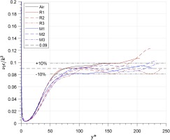
With the data for R1233zd(E) and MDM collected so tightly around the constant Cμ line across all cases, there is little evidence to suggest that real-gas effects have a significant impact on this value. A conclusion can therefore be made that the assumption Cμ=0.09 is still suitable in the standard two-function RANS model (k−ϵ and k−ω) within the outer layer region at y∗>70 for the organic fluids within this study.
Conclusions
This work studied the fully developed compressible turbulent channel flow of two organic fluids, R1233zd(E) and MDM, by means of Direct Numerical Simulation. Three cases for each fluid are set up at the same global Reynolds number (ReG = 4,880) and global Mach number (MaG = 2.25), and they are compared with an air baseline case. Three cases are set up for each organic vapour, representing thermodynamic states far from, close to and inside the supercritical region, and these cases refer to weak, normal and strong real-gas effect in each fluid.
The turbulent statistic parameters are analyzed and compared. The results show that the real-gas effect influences the averaged thermodynamic property profile. The averaged centre-to-wall temperature ratio is lower in the organic fluid with larger molecular weight, and this ratio will decrease as real-gas effect increases. The averaged wall-to-centre density ratio is also lower in the organic fluid with larger molecular weight, but increases as real-gas effect increases, which is reversed from the impact on averaged centre-to-wall temperature ratio.
The averaged centre-to-wall viscosity ratio is lower than 1, which is a kind of “liquid-like behavior”, when the real-gas effect is strong enough (in case R1 and M1). There exists a transition line (∂u/∂T)=0 for each organic fluid. when working condition is above this line (strong real-gas effect), the viscosity at channel centre is lower than at wall.
The real-gas effect does not influence the normal Reynolds stress in the streamwise direction, but it has an obvious impact on the other two normal Reynolds stress and the Reynolds shear stress. The peak values of the wall-normal Reynolds stress v′′v′′~ in real-gas cases are larger than that in air case by 7–20%, and the peak values of the spanwise Reynolds stress w′′w′′~ in real-gas cases are larger by 10–21%. The real-gas effect influences the viscosity profile, therefore, increases v′′v′′~ and w′′w′′~. The Reynolds shear stress u′′v′′~ is also increase by the real-gas effect since its peak value is 5–8% larger in two real-gas fluids than in air.
The turbulence kinetic energy dissipation ϵk in the viscous sublayer and buffer sublayer (y∗<30) can be impacted by the real-gas effect, which will increase as real-gas effect increases. The turbulence viscosity hypothesis within standard two-function RANS model (k−ϵ and k−ω) is checked in these two organic fluids, and the result shows that it is still suitable in the outer layer y∗>70 with a constant Cμ=0.09 for all real-gas cases, with an error in ±10%.
Nomenclature
Turbulent kinetic energy (J/kg)
Heat conduction (J/(m2s))
Specific entropy (J/kg·K)
Velocity in x direction (m/s)
Velocity in x direction (m/s)
Velocity in x direction (m/s)
Isobaric specific heat capacity (J/(kg·K))
Isochoric specific heat capacity (J/(kg·K))
Molecular weight (kg/kmol)
Turbulent kinetic energy generation rate (W)
Specific gas constant (J/(kg·K))
Compressibility factor (−)
Greeks
Turbulent kinetic energy dissipation rate (W)
Smallest length scale (m)
Kolmogorov length scale (m)
Length scale in temperature field (m)
Heat conductivity (W/(m·K))
Kinematic viscosity (m2/s)
Fundamental derivative (−)
Accents
Non-dimensional parameter
Reynolds-averaged mean parameter
Reynolds-averaged fluctuation
Favre-averaged mean parameter
Favre-averaged fluctuation