Introduction
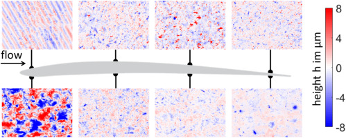
Rough surfaces influence the aerodynamics of turbomachinery, e.g. aero engines. In general, roughness increases losses in the flow due to higher production of turbulence: higher turbulence due to a change in momentum transfer between fluid and surface leads to higher losses. The increase of losses also leads to a decrease of the fluid’s velocity close to the wall and thereby an increase of the boundary layer thickness. Also other properties of the blade like the location of separation bubbles or the transition point are affected by the change of the boundary layer flow (Roberts and Yaras, 2005).
The velocity defect induced by the roughness leads to a deflection of the wake, and a change of incidence angle on the stage downstream. A disturbance of the incidence, for example in a compressor, can reduce the performance by up to 2.5% (Seehausen et al., 2020). Examples for the diverse types of roughness, found on worn blades of an airplane engine, are shown in Figure 1. The roughness depends on the location of the blade in the engine and on the position on the blade (Gilge et al., 2019a). In low-fidelity simulations like RANS, the boundary condition is modified to take the roughness of the wall into account. In the k−ω turbulence model by Wilcox (1988) for instance, the roughness is described by a single parameter, the equivalent sand grain roughness ks, to modify the ω boundary condition. The equivalent sand grain roughness is correlated with the roughness topology. Bons (2010) gives an overview about the many existing approaches to correlate ks with the profile of the rough surface. These correlations either use parameters calculated from linear surface height measurements (h=f(x)) or areal surface measurements (h=f(x,y)), as defined in various industrial standards (DIN EN ISO 4287, 2009; DIN EN ISO 25178-2, 2012).
Figure 1.
Examples of roughness measured on the blades of the third stage of a compressor adopted from (Gilge et al., 2019a). An extended collection of roughness measurements from worn compressor blades and a worn blisk can be found in (Gilge et al., 2019b).
To develop new models, or to improve the existing turbulence models and the ks correlations, results from experiments or direct numerical simulations (DNS) can be used. In recent years, an increased focus is set on the influence of the skewness parameter SSk, the effective slope ES or the arithmetic roughness height Sa. Experimental studies by Flack et al. (2020) and numerical simulations by Kuwata and Nagura (2020) show, that positively-skewed surfaces have a higher influence on the flow than negatively-skewed surfaces. The roughness peaks of positively-skewed surfaces reach further into the boundary layer and increase the drag and the turbulence production (Jelly and Busse, 2018). Flack et al. (2020) also show that the drag created by rough surfaces, is more sensitive to the root mean square roughness height when the surface is positively-skewed than negatively-skewed. Kuwata and Nagura (2020) show that the drag is equally sensitivity to the effective slope of the roughness elements. The effective slope ES is changed from ES=0.1 to ES=0.6 by compressing the roughness in the horizontal dimensions. The influence of the effective slope on the flow, measured by an decrease of the roughness function ΔU+, is not linear. For ES<0.4 a steady decrease of ΔU+ can be observed, getting smaller for ES>0.4. An explanation for this effect can be found when analyzing the composition of the total flow resistance, which consists of the viscous drag and the pressure drag. With an increasing effective slope, the ratio of pressure drag to viscous drag is increasing and becomes dominant for ES>0.4. Comparable observations are also made by Ahrens et al. (2021), who investigate the influence of the relative angle between the flow and the dominant direction of anisotropic rough surfaces. By changing the flow angle, the observed effective slope by the flow is changed and thereby the ratio of pressure to viscous drag.
This brief (and by far not full overview) of recent research shows the many influencing factors that need to be considered for modeling the influence of roughness on wall bounded flows. In this paper, further investigations into the influence of roughness skewness are conducted, with the aim to find a new or to improve an existing ks-correlation for rough surfaces found on aero engine blades. To investigate the influence of single roughness parameters independently, direct numerical simulations of systematically varied rough surfaces are conducted.
Systematically varied real roughness
Two roughness, found on compressor blades of a medium size high-bypass aircraft engine, are used as a basis for this investigation (Gilge et al., 2019b). An overview is shown in Figure 2. A confocal microscope is used to measure the surfaces height on equidistant scanning points (Δx+=Δy+=1.5). More information about the measurement and processing of the surfaces can be found in Gilge et al. (2019a) and Kurth et al. (2021). All physical distances s are non-dimensionalised by
Figure 2.
Base and mirrored roughnesses used for systematic variation of roughness density, height and skweness. Scaled for DNS with Reτ=395. (a) Reference Surface A (b) Mirrored Surface A (c) Mirrored Surface B (d) Reference Surface B.
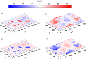
with uτ being the friction velocity, and ν being the kinematic viscosity of a smooth surface under the DNS flow conditions. Both reference surfaces are found on a blade from the third stage of a high-pressure compressor. reference surface A (Figure 2a) is found on the suction side and is dominated by deposits. reference surface B (Figure 2d) is found on the pressure side and was formed primarily by impacts. Both types of roughness are varied systematically to investigate the isolated influence of roughness skewness, height, and density. An overview for some parameters for all investigated surfaces is given in Table 1 in the appendix.
Table 1.
Roughness parameters of simulated surfaces.
| Base Roughness | Mirrored | Scaling Factor | |
|---|
| sfx | sfy | sfz | Sa+ | Sz+ | SSk | SKu | Esx | ksSa+ | ksSD+ | ksSDS+ |
|---|
| Reference | A | | 1 | 1 | 1 | 5 | 29.6 | 1.9 | 7 | 0.19 | 26 | 23 | 23.6 |
| A | x | 1 | 1 | 1 | 5 | 29.6 | −1.9 | 7 | 0.19 | 26 | 24 | 8.6 |
| B | | 1 | 1 | 1 | 6.5 | 31.3 | 0.96 | 3.5 | 0.15 | 33.8 | 21 | 15 |
| B | x | 1 | 1 | 1 | 6.5 | 31.3 | −0.96 | 3.5 | 0.15 | 33.8 | 19.8 | 7.4 |
| Roughness Height | A | | 0.8 | 0.8 | 0.8 | 4.1 | 23.7 | 1.9 | 7 | 0.19 | 21.3 | 18.5 | 18.9 |
| A | x | 0.8 | 0.8 | 0.8 | 4.1 | 23.7 | −1.9 | 7 | 0.19 | 21.3 | 19.4 | 6.9 |
| B | | 0.8 | 0.8 | 0.8 | 5.2 | 25 | 0.96 | 3.5 | 0.15 | 27 | 16.8 | 12 |
| B | x | 0.8 | 0.8 | 0.8 | 5.2 | 25 | −0.96 | 3.5 | 0.15 | 27 | 15.8 | 5.9 |
| A | | 1.2 | 1.2 | 1.2 | 6.1 | 35.5 | 1.9 | 7 | 0.19 | 31.7 | 27.7 | 28.4 |
| A | x | 1.2 | 1.2 | 1.2 | 6.1 | 35.5 | −1.9 | 7 | 0.19 | 31.7 | 29.1 | 10.4 |
| B | | 1.2 | 1.2 | 1.2 | 7.8 | 37.6 | 0.96 | 3.5 | 0.15 | 40.6 | 25.3 | 18 |
| B | x | 1.2 | 1.2 | 1.2 | 7.8 | 37.6 | −0.96 | 3.5 | 0.15 | 40.6 | 16.8 | 8.8 |
| Roughness Density | A | | 0.8 | 0.8 | 1 | 5 | 29.6 | 1.9 | 7 | 0.23 | 26 | 29.3 | 30 |
| A | x | 0.8 | 0.8 | 1 | 5 | 29.6 | −1.9 | 7 | 0.23 | 26 | 30.7 | 11 |
| B | | 0.8 | 0.8 | 1 | 6.5 | 31.3 | 0.96 | 3.5 | 0.18 | 33.8 | 26.8 | 19.1 |
| B | x | 0.8 | 0.8 | 1 | 6.5 | 31.3 | −0.96 | 3.5 | 0.18 | 33.8 | 25.2 | 9.37 |
| A | | 1.2 | 1.2 | 1 | 5 | 29.6 | 1.9 | 7 | 0.17 | 26 | 18.9 | 19.4 |
| A | x | 1.2 | 1.2 | 1 | 5 | 29.6 | −1.9 | 7 | 0.17 | 26 | 20 | 7.1 |
| B | | 1.2 | 1.2 | 1 | 6.5 | 31.3 | 0.96 | 3.5 | 0.12 | 33.8 | 17.3 | 12.3 |
| B | x | 1.2 | 1.2 | 1 | 6.5 | 31.3 | −0.96 | 3.5 | 0.12 | 33.8 | 25.2 | 9.4 |
Isolation of roughness skewness
The skewness (SSk) of the roughness is a parameter used to quantify, whether a roughness consists primarily of hills (SSk>0; reference surface A) or valleys (SSk<0; reference surface B). By mirroring the reference surface on the x-y-plane, the skewness is inverted. This has the great advantage that all other parameters change little to none.
Variation of roughness height
To change the roughness height without changing it’s density, all dimensions are multiplied by a scaling factor sf. For this paper, the base and the mirrored roughness were varied with scaling factors of sf=0.8 and 1.2 respectively. The change of roughness height is influencing roughness parameters like the mean roughness height Sa or the equivalent sand-grain roughness ks. Other parameters like the skewness SSk of the roughness or the effective slope Es are not changed.
Variation of roughness density
By multiplying only the horizontal roughness dimensions (x and y) by a scaling factor sf, the density of the roughness is changed. Again, the base and mirrored roughness were varied with scaling factors of sf=0.8 and 1.2 respectively. Because the roughness height does not change, parameters like the mean roughness height Sa and skewness SSk do not change. The equivalent sand-grain roughness height ks only changes, if it is based on the shape and density parameter but not, if it based on the mean roughness height Sa.
Numerical setup
In this study, an immersed boundary method (IBM) is adopted for direct numerical simulation (DNS) of the flow over the rough surface. This method has some advantages over the conventional body-fitted approach. Firstly, the mesh is regular with perfect quality, being independent of the immersed body. Secondly, the mesh can also be used for other surfaces, simply because the introduction of the surface involves nothing but immersion in the computational domain. Last but not the least; the generation of the mesh requires very little human effort. The IBM approach used in this paper is provided in foam-extend-4.0. It is based on the polynomial fitting of the solution on the IB cells concerning the boundary condition on the wall. A detailed explanation of the method can be found in Senturk et al. (2019).
The CFD tool used, foam-extend-4.0, is based on a cell-centered finite volume discretization. For the incompressible solver based on icoFoam, Gauss linear scheme and backward temporal discretization are chosen, resulting in second-order accuracy both in time and space. PISO algorithm is used for the solution of the incompressible flow equations. For all the simulations, a maximum CFL number smaller than 0.5 is ensured.
A channel setup is convenient to investigate the flow over a roughness patch because the friction velocity Reynolds number
can easily be set through the incorporation of a constant body force in the momentum equations. Hence, the drag on the surface is balanced by this flow-driving force as long as the flow is fully developed. The boundary layer thickness δ is fixed by half channel height, where symmetric conditions are imposed. Moreover, periodicity is imposed on the lateral boundaries to enable not only the use of a smaller domain but also the use of spatial averaging for better flow statistics. On the bottom wall, the roughness patch is immersed in the mesh ensuring no-slip condition. The mean height of the surface corresponds to the z=0 plane (Figure 3). The periodicity of the roughness patch is ensured by using a linear blending function to blend 10% of the roughness patch on the borders. The structured computational mesh is generated using constant spacing in both of the lateral directions.
Figure 3.
Double-infinite channel with rough surfaces on bottom wall. The channel is symmetric in wall-normal direction with the gray plane being the symmetry plane.
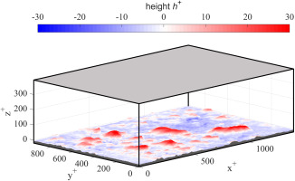
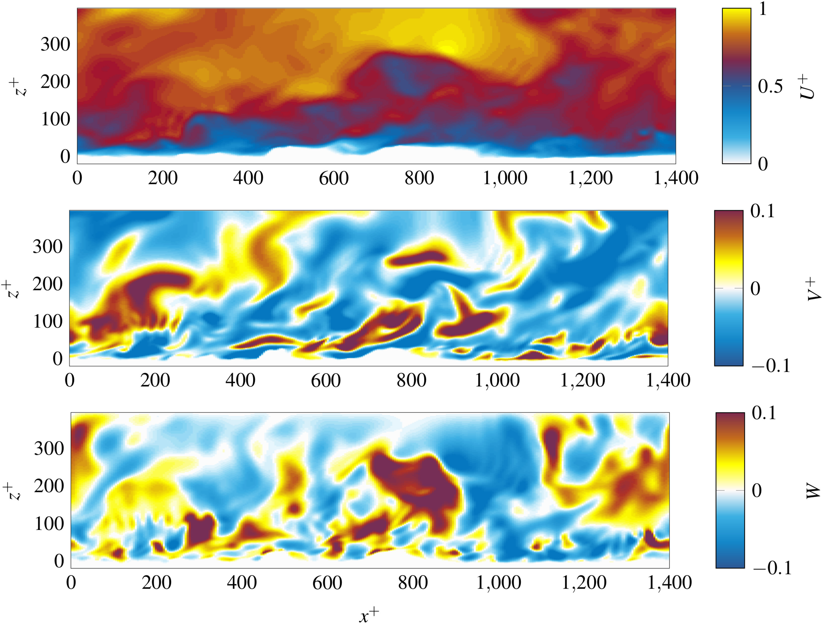
The mesh consists of nX×ny×nz=200×138×160≈4.4⋅106 cells, resulting in a lateral mesh spacing of Δx+=Δy+=7.3. The mesh resolution study included in Kurth et al. (2021) shows, that this resolution still allows for accurate DNS results. In the wall-normal direction, the channel is split into three blocks: the IB block with a constant spacing z+≈0.9, the transition block with a growth rate of less than 6%, and the core block with a constant spacing of z+≈4.9. In this study, a friction Reynolds number of Reτ≈395 is enforced for all of the simulations. As soon as the flow is developed, statistics are collected for a sufficient amount of convection time. The statistics are then averaged both spatially and temporally. Figure 4 shows the three momentary velocity components at a time step for the vertical mid-plane of the computational domain, as an example for the simulation results. The roughness can be recognized at the bottom of the surface plot. It is influencing the flow by deflecting the flow in vertical and horizontal direction.
Figure 4.
Excerpt of DNS simulation of Reference Surface A. The three momentary velocity components at the vertical mid-plane of the computational domain are shown.

The DNS-IBM approach is validated with the Reτ≈180 channel setup on a smooth surface with the highly resolved DNS results, as well as on a rough surface. All the validation results can be found in the previous communication Kurth et al. (2021).
Results
During the simulation, the friction velocity Reynolds number (Equation 2) is kept constant by applying a constant body force on the fluid. An increase of losses by the roughness is therefore shown as a decrease of the mass flow. In the velocity profiles, shown in Figure 5, this decrease of mass flow is reflected by a decrease of velocity. In comparison with the results of a smooth channel DNS, the simulations with a roughness show a velocity deficit ΔU+. Despite keeping roughness parameters other than the skewness constant, both types of roughness show considerably different velocity deficits. This confirms the importance of roughness skewness for building or improving a ks-correlation.
Figure 5.
Boundary layer profile of Reference Roughness A and Mirrored Roughness A compared to smooth channel DNS results by Moser et al. (1999). The velocity defect ΔU+ is defined as difference between the velocity profiles in the log-law region.
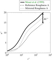
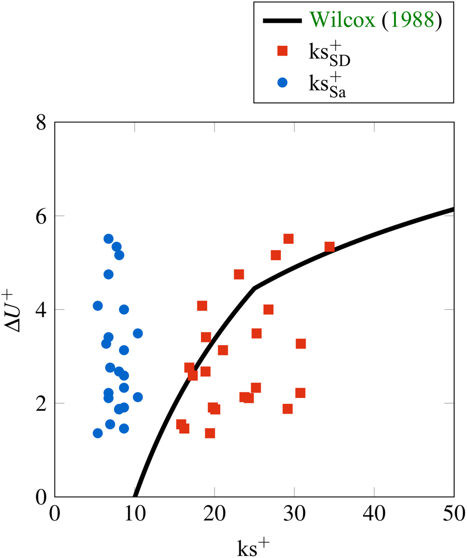
Figure 6 shows the velocity deficit ΔU+ and the ks+ value, calculated with two different correlations, for each investigated surface. The correlation by Hummel et al. (2004)
Figure 6.
Comparison of ks+ values calculated with the correlation by Hummel et al. (2004) (ksSa+) and Bons (2005) (ksSD+) to the velocity defect calculated from the DNS results.
uses the mean roughness height
The correlations by Bons (2005)
use the shape and density parameter
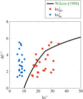
by Dirling (1973). The shape and density parameter evaluates the density of the roughness elements and the gradient (shape) of the roughness elements. For the roughness height k the maximum roughness height Sz is used. Both correlations can’t predict the equivalent sand grain roughness ks correctly. The ks+ values calculated with the correlation by Hummel et al. (2004) have less variation, because it is only based on the mean roughness height Sa. The ks+ values calculated with the correlation by Bons (2005) span a broader region. However, both correlations fail, as very similar ks+ values are calculated despite the significantly different velocity deficits ΔU+.
Within the k−ω− turbulence model by Wilcox (1988), the wall function is defined by
The constant B depends on the roughness of the wall. For smooth surfaces it is given as
For rough surfaces it is given as
with
The velocity difference for a given equivalent surface roughness ks+ can be calculated by the difference of the smooth (US+) and rough (UR+) wall function:
The accuracy of a ks-correlation can be evaluated by the fit of its prediction of ks+ to Equation 11. The coefficient of determination is R2=0.02 for the correlation by Hummel et al. (2004) and R2=0.11 for the correlation by Bons (2005).
Modelling the influence of skewness
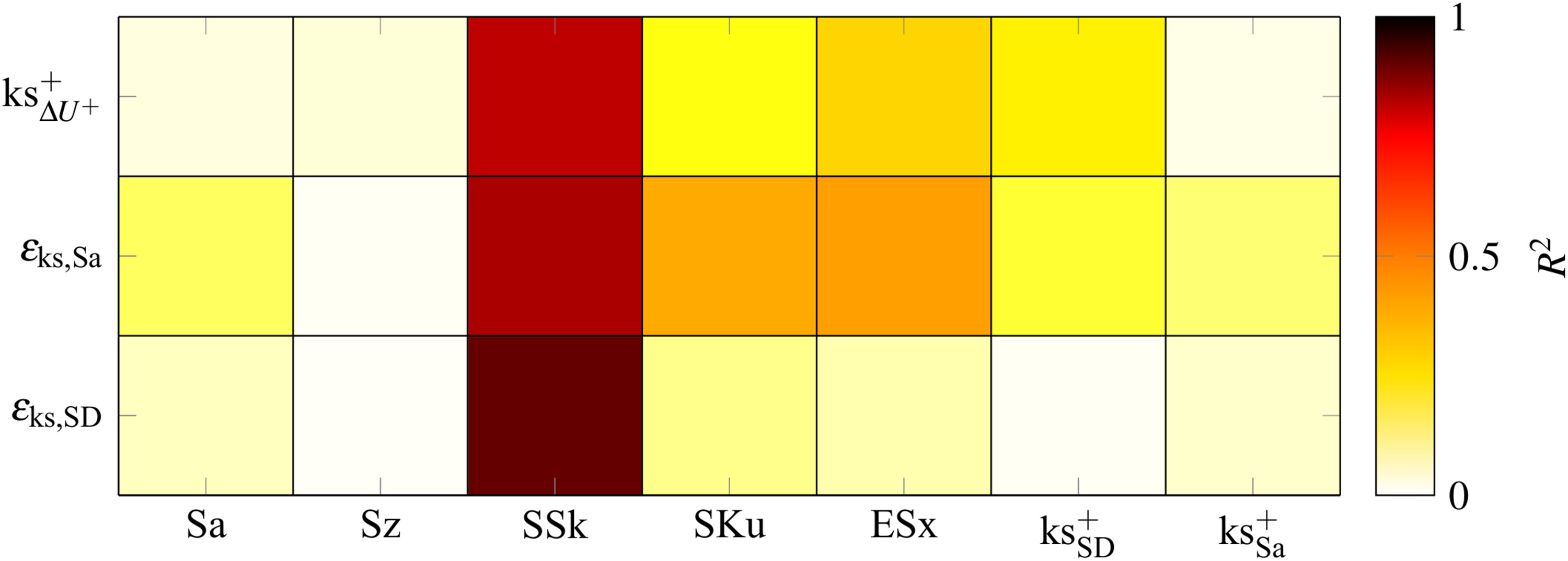
A correlation matrix is used to identify or improve correlations from the roughness geometry to the DNS results. Figure 7 shows an excerpt of a correlation matrix for the given DNS results. Roughness parameters, calculated from the roughness geometry, are listed on the abscissa. On the ordinate, values deduced from the DNS are listed. Solving Equation 11 for the equivalent sand grain roughness ks+ results in a function to calculate the sand-grain roughness ksΔU+, that must be set as roughness in the low order simulation to achieve the same velocity deficit ΔU+ as observed in DNS:
Figure 7.
Excerpt of correlation map for roughness parameters and DNS results.

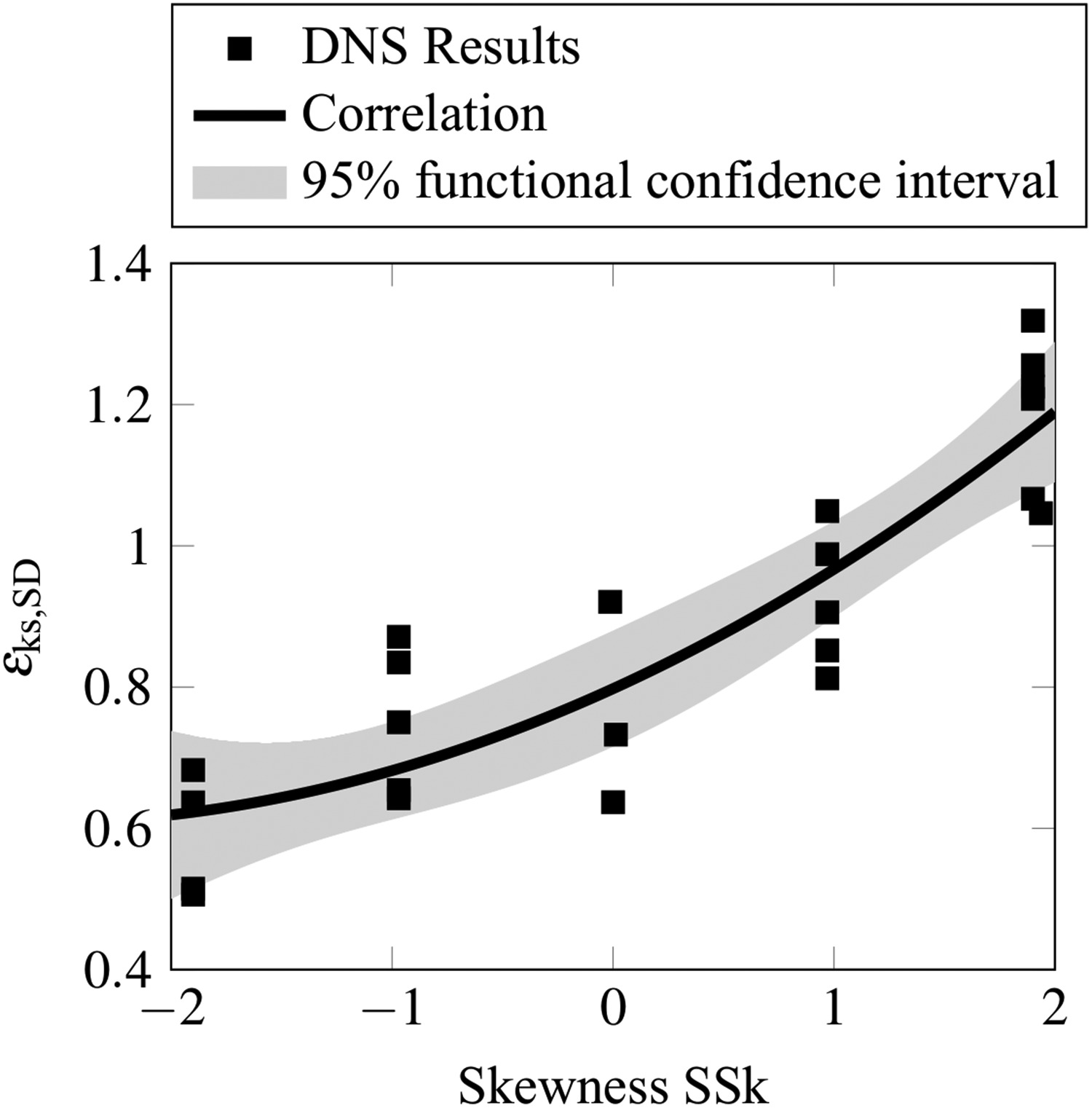
The coefficient of determination R2 of the 2nd order polynomial correlation fit is color coded: the darker the color, the better the fit. It can be seen, that no roughness parameter except of the skewness shows a good fit to the observed DNS results. The best correlation (R2≈0.93) is found for the skewness to the ratio of ksSD+ to ksΔU++. Figure 8 shows the correlation function
Figure 8.
Correlation function for skewness to relative ratio of the ks-correlation based on shape and density parameter and the ks-value based on velocity deficit ΔU+ from DNS results.

Most DNS results are within the 95% functional confidence interval shown as a gray shadow. Based on the found correlation, the ks-correlation based on the shape and density parameter can be improved.
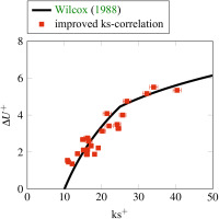
The equivalent sand grain roughness
calculated from the roughness geometry with the correlation based on the shape, density and skewness parameter is shown in Figure 9. The factor ϵks,SD can be seen as a scaling factor, depending on the skewness of the roughness. For large positive skewness, the scaling factor is close to 1. The ks-value is about the same as calculated with the shape and density parameter. For smaller and negative skewed roughness profiles, the ϵks,SD is <1. The equivalent sand grain roughness calculated with the shape an density parameter is decreased. A great improvement in predicting the influence of the investigated roughness is achieved. The coefficient of determination for the improved correlation is R2=0.90, compared to R2=0.11 for the correlation by Sigal and Danberg (1990). The equivalent sand grain roughness of all surfaces can be calculated to predict the correct influence on the flow even with RANS.
Figure 9.
New ks-correlation based on Shape-, Density- & Skewness-Parameter.
Conclusions
The aim of this investigation is to improve the equivalent sand grain roughness (ks) correlation for surfaces from aero engines. To achieve this, direct numerical simulations (DNS) of channel flows with systematically varied rough surfaces are carried out at a friction Reynolds number of Reτ=395. Two rough surfaces are taken from the compressor blades of a medium size high bypass aircraft engine. They are varied by stretching and compressing to change the roughness density and height. Additionally, all rough surfaces are mirrored on the horizontal plane to change their skewness without changing any other parameters. The mirrored surfaces are found to have a significantly different effect on the flow, even though the same equivalent sand grain roughness is calculated by existing correlations. The DNS results are correlated with various roughness parameters. The best results are achieved when correlating the skewness of the roughness with the quotient of the ks value based on the shape and density parameter and the ks value based on the velocity deficit from the DNS. Extending the correlation based on the shape and density parameter, with a function based on the skewness parameter, the ks-correlation is improved from R2=0.11 to R2=0.90. The improved ks-correlation needs to be validated in future investigations.
Nomenclature
effective slope in x-direction (A−1∫∫A∂h∂idA)
equivalent sand grain roughness (equ. 12, 3, 5)
normalized equivalent sand grain roughness (uτ⋅ks⋅ν−1)
shear stress Reynolds number (uτ⋅δ⋅ν−1)
coefficient of determination (−)
mean roughness height (A−1∫∫A|h|dA)
kurtosis of height values (Sq−4A−1∫∫Ah3dA)
sknewess of height values (Sq−3A−1∫∫Ah3dA)
root mean square roughness height (A−1∫∫Azh2(x)dA)
maximum roughness height (−)
friction velocity (τW⋅ρ−1)
normalized velocities (u⋅uτ−1)
normalized spatial coordinates (uτ⋅x⋅ν−1)
correlation function (ksSD+/ksΔU++)
shape and density parameter (−)