Effects of different blade loading strategies applied to low specific speed tube-axial fans

Current industrial fans belonging to the tube-axial type offer the best performance for specific speeds higher than 6. For specific speed higher than 7.5, it is widely demonstrated that the performance requirements and efficiency of fans designed using the free-vortex blade load distribution can be matched, when not exceeded, by using other blade load distributions, also with advantage in terms of fan size reduction. On the other hand, the large number of free-vortex designs populating the vane-axial industrial fan type, suggests that the advantage associated with blade load distributions other than free-vortex reduces as specific speed decreases and vanishes at specific speeds lower than 6. This work presents and compares three fan designs conceived by the authors for specific speed approximately equal to 4.3. The fans feature a hub-to-tip ratio equal to 0.5 and differ to each other only in the blade load distribution that varies from free-vortex to rigid-body, passing through the constant-swirl one. The aims of the work are to quantify the pros and cons associated with the considered blade loading distributions, to identify the blade loading concept best suited to the range of specific speeds where hub-to-tip ratios equal to 0.5 are recommended for tube-axial fans and, to assess the capability of the design method originally suggested by the authors for fans with low hub-to-tip ratio. For this purpose, CFD-RANS analyses were carried out to preliminarily characterise all three proposed designs and identify the most efficient one. The most promising solution was manufactured by rapid prototyping, in the 315 mm diameter size, and tested according to ISO 5801. The results demonstrate that the constant-swirl blade loading distribution offers good performance even at specific speeds close to the lower extreme of the usual tube-axial industrial fans application range and can be successfully realised using the improved version of the authors’ method presented here.

Introduction

The preliminary design workflow of any turbomachine starts with the conceptual design, followed by the basic sizing of the blade (Csanady, 1964). The former fixes both the machine type – mostly related to the meridional topology (e.g., axial, mixed-flow, radial…) – and the diameter and speed of the rotor. The latter defines the rotor blade geometry, usually as envelope of two-dimensional profiles placed on a series of revolved surfaces approximating the real streamsurfaces that develops within the rotor (Lewis, 1996).

Conceptual design

It can be effectively pursued exploiting design charts that collect the maximum efficiency values achievable by each turbomachine type as a function of the dimensionless performance parameters desired at rated operation – e.g., Cordier diagrams for hydraulic machines (Cordier, 1953) and Smith charts for axial turbines (Smith, 1965) or axial compressors (Casey, 1987). The dimensionless parameters commonly used in the axial-flow fan conceptual design rely on appropriate combinations of nominal volume flow rate (q_v), increase of mechanical energy per unit mass (ΔH), rotor diameter (D) and rotational speed (ω), which define either the flow and pressure coefficients pair at design (Φ_d and Ψ_d, respectively), or the specific speed and specific diameter pair (Ω and Δ). In particular, the former and the latter pairs are defined as reported in Equation 1 and relate to each other in accordance with Equation 2 (Csanady, 1964).

(1)

Φd=qv/(ωD3);Ψd=ΔH/(ω2D2)Ω=ωqv0.5/ΔH0.75;Δ=DΔH0.25/qv0.5

(2)

Φd=1/(ΩΔ3);Ψd=1/(Ω2Δ2)Ω=Φd0.5/Ψd0.75;Δ=Ψd0.25/Φd0.5

Obviously, the practical effectiveness of design charts built from statistical analysis of real machines data – as for the original Cordier diagrams (Cordier, 1953) or the analogous ones suggested by (Eck, 1973) – depends on the degree of design improvement achieved by the turbomachine type after the date such charts were built. In fact, the advancements in axial-flow fan technology during the last four decades were not marginal, as demonstrated in (Masi et al., 2022a) by comparing the dimensionless charts of fan performance and efficiency updated to year 2020 catalogues data to the corresponding year 1980 charts collected in (ESDU, 1980). However, regardless of the charts update issue, the major weakness of conceptual designs based on such charts relies on the ever-missing information on the rotor blade loading distribution, which is crucial for the subsequent sizing of the blade. In fact, with a fixed velocity distribution upstream of the rotor and fixed work done by the blade, different blade loading distributions result in different spanwise distributions of the velocity diagrams, that translate to different losses and, accordingly, different fan efficiencies. Thus, the main practical consequence of an arbitrary selection of the blade loading distribution is that the basic sizing of the blade many times fails to meet the conceptual design expectations.

Basic sizing of the blade

Considering the issues related with design charts built from catalogue data, designers can find support for the basic sizing of the blade in additional resources. The timeless semi-empirical Baljé charts (Baljé, 1981), made available more than forty years ago for most turbomachines (sadly not for low-speed tube-axial fans), are a first example of such resources. The CFD-based Smith-like charts, recently proposed by (Smyth and Miller, 2021) for compressor rotors, are another example. In fact, charts from both examples are based on the “a priori” assumption of a specific blade loading distribution, which eliminates the need for arbitrary assumption but, at the same time, does not assure that the applied blade loading concept leads to the most efficient blade design. Being well-aware of this limitation, Baljé compared two optimum efficiency charts of rotor-straightener blowers with shrouded rotors (Baljé, 1981) that he obtained assuming alternatively free-vortex (FV) and rigid-body (RB) blade designs and showed the remarkable sensitivity of maximum efficiency and corresponding aerodynamic performance to the blade loading distribution. Such sensitivity was implicitly confirmed also by (Lewis, 1996) when he underlined the noticeable departure from the Cordier line of several good design axial fans included in the ESDU report (ESDU, 1980). In fact, the effect of blade loading distribution on global fan performance is a long-time-investigated topic, which have not yet been definitely quantified. For example, (Kahane, 1948) designed three 0.69 hub-to-tip ratio (ν) fan rotors with Φ_d = 0.093, two of them with RB blade loading distribution, and one with constant-swirl (CS) at the rotor exit. The RB blade loading distribution outperformed the static pressure rise of the CS distribution by approximately 13%, but at the cost of an approximately 7% lower static efficiency. Another example, at the opposite extreme of ν values employed in low-speed axial-flow fan designs, is the 1.845 mm diameter propeller fan with ν = 0.14 and RB-like blade design, whose geometry and performance data are reported in (Wang and Kruyt, 2020). According to the data rearrangement presented in (Masi et al., 2022b), the fan achieves 75% η_aer in operation at Φ_d = 0.0728 and Ψ_d = 0.0124, with flow separation at the blade root. In (Wang and Kruyt, 2022), the same fan design was compared to different designs implementing other blade loading distributions. According to the CFD results, the FV blade load distribution emerged as best trade-off between performance and efficiency, if an increase up to 0.3 is allowed for ν. Unfortunately, this study lacks experimental assessments. Vice versa, experimental data were reported in (Masi et al., 2022b), where the same RB propeller fan design was taken as benchmark to verify the efficiency achievable by a roughly-CS rotor designed to operate at the same Φ_d, with no separation at the blade root. The experimental data measured at different values of the blade positioning angle for the CS prototype scaled to the 315 mm diameter size, demonstrated that the CS design, is capable of achieving η_aer in excess of 73% and Ψ_d ≈ 0.089, if its blades are appropriately positioned to match Φ_d at maximum efficiency operation. Considering the efficiency detriment expected by the 6-times smaller size of the CS prototype, it is expected that a full-scale version of this machine could equal (and likely exceed) the η_aer of the RB design at the cost of an approximately 30% lower Ψ_d, in qualitative agreement with (Kahane, 1948).

Recent findings on tube-axial fan preliminary design

The present availability of appropriate computational resources makes artificial intelligence (AI) a feasible alternative to obtain design charts. In fact, approximately 40 years after Baljé, (Bamberger and Carolus, 2020) presented Baljé-like charts they referred to as “practical fan efficiency limits charts”, obtained using a RANS-CFD-based optimisation method coupled with parametrised fan geometries. Unfortunately, such charts still do not disclose any information on the blade design, except for the statement “…in order to minimize the exit losses…” of fans with outlet guide vanes “…the load distribution is isoenergetic…”, which is reminiscent of a previous work dealing with the aerodynamic analysis of three optimised tube-axial fans (Bamberger and Carolus, 2015). These fans fall on the Cordier line populated with designs defined by an artificial neural network (ANN)-based optimisation technique trained by approximately 13,000 steady-state CFD-RANS simulations (Bamberger and Carolus, 2014) and, according to those authors, demonstrate that FV blade loading roughly resembles the actual blade loading of any optimum efficiency tube-axial fan design falling on the Cordier line. This outcome is compatible with the previously reported findings of (Wang and Kruyt, 2022) and (Masi et al., 2022b), according to which the most efficient blade loading distribution for very-low-ν fans could be the FV one, followed by CS and RB, in that order. A more useful application of AI to fan preliminary design is documented in (Angelini et al., 2019), where new “multidimensional Balje charts” were suggested. These design charts, derived from more than 7,000 axi-symmetric RANS simulations, were driven by optimisation techniques not much different than those used in (Bamberger and Carolus, 2014, 2020), but were tailored to a more design-oriented result. In fact, the suggested charts enlarge the set of dimensionless design parameters included in the original Baljé charts by addition of other contour lines for combined pairs of blade design parameters (e.g., ν and blade solidity, aspect ratio and twist). Unfortunately, this promising attempt to update tube-axial fan preliminary design charts was not developed further to become a practical design tool and, at present, it does not allow the designer the direct extraction of the best blade loading concept.

General fan research gap

To sum up, this brief literature overview on fan preliminary design leads to conclude that: (i) there is still a lack of solid confirmation on the existence of an optimal blade loading distribution valid for all tube-axial fan rotors, regardless of the application; (ii) there are no explicit identifications of the Ω range each blade loading distribution is better suited to; (iii) there are no definite indications of the quantitative advantages and limitations of different blade loading distributions for fan rotors with ν close to the maximum values generally found suitable for industrial tube-axial fans.

Authors’ fan research gap

The design method for tube-axial fans with CS blade loading distribution, formalised by the authors a few years ago (Masi and Lazzaretto, 2019a,b) – hereafter referred to as ML method – did not yet demonstrate its reliability for designs with ν > 0.4. Moreover, the method still lacks a criterion to account for the blade tip gap effect on the radial migration of the meridional flow within the rotor vanes, and a “not-subjective way” for assigning the local incidence value to the aerofoil sections chosen as skeleton of the blade during the design process.

Aims of the work

To contribute towards filling the authors’ fan research gap previously reported and, mostly, to contribute to item (iii) of the general fan research gap with a quantitative comparison of the effect of different blade loading distributions on a low-Ω tube-axial fan design with ν = 0.5.

Structure of the paper

The first Section is subdivided in three Sub-sections each one focusing on the details of the blade aerodynamic design of one of the three fans designed for this work. In fact, the three fans were designed for the same aerodynamic requirements – voluntary fixed to permit achieving good efficiency designs with ν = 0.5 – and differ from each other only in the blade loading distribution. The second Section presents the CFD model and the experimental setup used to assess the fan designs. The CFD validation of the three designs is the subject of the third Section, whereas the fourth Section deals with the results. In particular, the latter provides the comparison of the global aerodynamic performance predicted by CFD for the three designs and the experimental data measured for the CS design manufactured by rapid prototyping, and a discussion of the obtained results. Finally, the Conclusions summarise the major findings of the work.

Novelty and originality

To the best of the authors’ knowledge, this is the first contribution in the low-speed axial-fan literature that presents a comprehensive comparison of the aerodynamic performance obtained by three tube-axial fans with ν = 0.5 differing from each other only in the blade loading distribution. Also, the ML method is used for the first time to design a tube-axial fan with ν = 0.5. Moreover, the version of the method used here evolves the original formulation in the assignment of the local incidence of the aerofoil sections and embeds an original empirical criterion to account for the tip gap effect on the obliquity of the meridional flow.

Methodology

Three tube-axial fans sharing the same rotor size and speed were designed to fulfil the same duty requirements with alternatively the FV, RB, or CS blade loading distributions. Furthermore, to reduce as much as possible the influence on the global aerodynamic performance due to design differences not strictly associated with blade loading, the designs share also:

The same ν value – to obtain the same velocity diagrams upstream of the rotor blading and virtually the same average relative velocity of the bulk-flow in the blade passage – set equal to 0.5 as representative of the maximum value commonly used in tube-axial industrial fans.
The same (Φ_d, Ψ_d) pair, equal to (0.075, 0.025) – specifically chosen to obtain fan designs with the same Ω ≳ 4 – appropriate to achieving the maximum η_aer practically expected from state-of-the-art tube-axial fans with ν = 0.5 (Masi et al., 2022a).
Much the same wall surface area – to equalise the wall friction effects – owing to the selection of the same blade counts (z = 12) and aspect ratio (AR ≈ 1.7).
The same aerofoil sections family – to obtain blade designs starting from the same aerodynamic performance potential – namely, the F-Series (Wallis, 1993) aerofoil with the same dimensionless thickness (th/l = 10%) and nose droop (d/l = 3%), when not specified differently.
The same aerofoil section operating conditions at the fan design duty – to obtain ideally the same stall margin – set at the maximum value of C_L/C_D.

In the absence of inlet guide vanes upstream of the rotor, all classical design methods, as for example (Carolus and Starzmann, 2011), generally assume that the absolute velocity distribution at the rotor entrance is purely axial and spanwise constant, and that the flow is in radial equilibrium just upstream and downstream of the rotor blades. This permits the univocal definition of the velocity triangles compliant with the chosen blade loading distribution. To make easier the comprehension of symbols and notations used hereinafter, Figure 1 shows a sketch of a tube-axial fan meridional view including the notation used for the main geometrical parameters and an example of the local inlet and exit velocity triangles. These are reported in dimensional form (on the left) and in the dimensionless counterpart (on the right).

Figure 1.

Sketch of a tube-axial fan meridional view with the main geometrical parameters and the local velocity triangles in dimensional (left) and dimensionless (right) form.

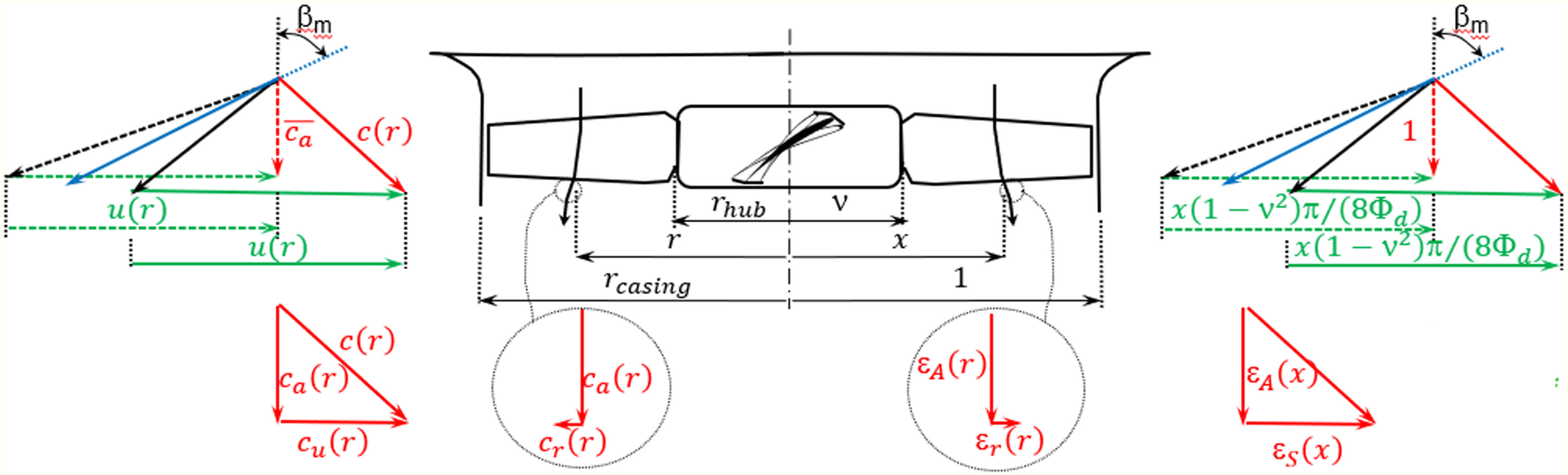
https://journal.gpps.global/f/fulltexts/204815/JGPPS-00263-2024-01.01_min.jpg

Note that the local tangential, axial, and radial (if present) absolute velocity components (c_u, c_a, and c_r in that order) find their dimensionless equivalents in the swirl coefficient (ε_S), axial velocity ratio (ε_A) and radial velocity ratio (ε_R) defined after (Wallis, 1993), as:

(3)

εS(x)=cu(x)/ca¯;εA(x)=ca(x)/ca¯;εR(x)=cr(x)/ca¯

where ca¯ and x are the average axial velocity in the blade channel and the dimensionless radial coordinate, respectively.

The next three Sub-sections present the basic sizing process of the FV, RB, and CS rotors blade, in that order, focusing on the major differences existing between the three processes. In fact, all the three design processes follow the three general steps that are described in detail in Appendix A and that are listed as follows:

Definition of the velocity diagrams that fulfil the fan aerodynamic performance requirements.
Specification the aerofoil sections that makes possible the work exchange associated with the velocity diagrams.
Quantification of the blade stagger.

In particular, the FV and RB blades were obtained by application of the “Kahane-Wallis” method (KW hereafter), as formalised in (Downie et al., 1993), whereas the CS blade was obtained by application of a slightly modified version of the ML method formalised in (Masi and Lazzaretto, 2019a,b). The latter evolves the KW method in order to better account for the radial flow migration in the specific case of a CS blade loading design that keeps the same aerofoil section and l all along the blade span.

Free-vortex design

Since both the work exchange and the axial velocity component assume spanwise constant values in FV designs, that means ε_S(x) ∝ x⁻¹, the first of the three design steps reported in Appendix A reduces to the assumption of ε_S(x) = 0.608/x (being ε_A(x) = 1) and 65% as guess value for η_aer at design operation, based on the total-to-static efficiency (η_TS) expected by (Bamberger and Carolus, 2015). These assumptions lead to the preliminary estimate of the expected pressure coefficient (Ψ_ext) obtained by the Euler work equation being rearranged as reported in Equation 4.

(4)

Ψext=xεS(x)2πΦd1−v2ηaer=0.025(≈Ψd)

To perform the second design step, Equation A2 was applied, neglecting all the drag coefficients and also neglecting, at first, the mutual interference between adjacent blades. This allowed for the determination of the spanwise distribution of the loading factor (σC_L). At the blade root, the latter resulted in a value equal to 1.44. High σC_L values at the blade root – where σ reaches values possibly well in excess of unity - should be fulfilled with relatively high C_L values to limit the penalisation introduced by the mutual interference between adjacent aerofoils. According to (Downie et al., 1993), for F-series aerofoil sections, it is not recommended to exceed a value of 1.3 for C_L, which is attainable with a camber (θ) slightly lower than 40° and attack angle (α) equal to 2° (after inclusion of the nose droop). The spanwise distribution of C_L was fixed to decrease from 1.3 up to 0.7 moving from the blade root to tip, considering that the FV blade design strongly reduces the aerodynamic load demand of aerofoil sections towards the blade tip. The spanwise distribution of α corresponding to such a C_L distribution permitted a preliminary estimate of ξ via Equation A3. The latter is necessary to estimate K_i, from the chart included in (Wallis, 1993), and obtain a σ distribution very close to the final one, using the following simplified and rearranged form of Equation A2.

(5)

σ=2εScos⁡(βm)CL(α)Ki(σ,ξ(βm,α))

The final spanwise distribution of ξ, that is the outcome of the third design step, was obtained after a few iterations of Equations A3 and 5, necessary to converge to the final σ and K_i values.

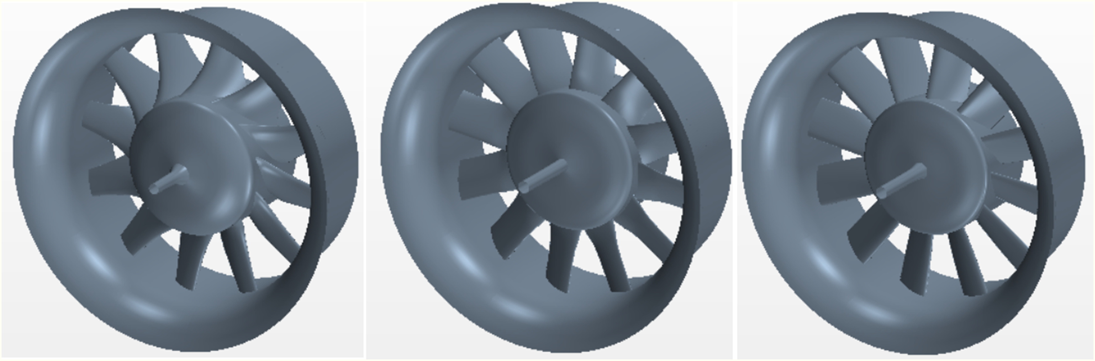
Finally, according to the fixed blade counts (12), the chord length distribution l(x) continuously decreases from 76.8 mm to 30.4 mm (moving from the root to tip), if the fan is manufactured with D = 315 mm. A view of this FV design fan is shown in the left frame of Figure 2.

Figure 2.

Perspective views of the FV (left), RB (middle), and CS (right) fan designs.

https://journal.gpps.global/f/fulltexts/204815/JGPPS-00263-2024-01.02_min.jpg

Rigid-body design

The non-uniform spanwise distribution of the work exchange imposed by the RB vortex distribution (ε_S(x) ∝ x) leads to the major implication that the higher the Ψ_d requirement is, the higher the minimum ν that allows operation without flow separation at the hub is. In fact, very few trials were necessary to state the impossibility to fulfil the present Ψ_d requirement without flow separation at the hub when ν = 0.5. It was therefore decided to increase the value of ν to 0.6 for the aerodynamic calculations, hereafter referred to as the “aerodynamic” hub-to-tip (ν_aero). This means assuming that the separation and flow reversal occurring at the “solid” ν is confined within a region that extends up to ν_aero, where a slip surface develops and behaves as a frictionless hub, at the cost of recirculation losses that penalise η_aer. The latter is therefore assumed equal to 50%. The additional assumptions of η_loc(x) = 0.85, as suggested in (Downie et al., 1993), and ε_S(x) = 0.875x permit the completion of the first design step, and specifically to:

Determine ε_A(x) from the radial equilibrium condition stated by Equation 6.
(6)
εA(x)=1−2⋅0.875(x2−x02)[0.875−ηloc(x)π(1−vaero2)8Φd]
where x₀ = 0.803 is the dimensionless radius at which ε_A reaches the unit value (obtained by fulfilling the flow continuity constraint across the fluid volume swept by the fan rotor).
Estimate Ψ_ext from the mass flow weighted integration of the local work exchange, as reported in Equation 7.
(7)
Ψext=∫vaero1⁡[xεS(x)2πΦd1−vaero2ηaerεA(x)]xdx∫vaero1⁡εA(x)xdx=0.024(≈0.97Ψd)

The second design step, as per FV design, was performed by application of Equation A2 in the simplified form that neglects all the drag coefficients and the mutual interference between adjacent aerofoils. For any non-FV design case, such an equation is written as:

(8)

σCL(α)=2εScos⁡(βm)0.5(1+εA)

The omission of K_i from Equation 8 is justified by the fact that in a RB blade design σC_L assumes its minimum value at the blade root (usually rather low, e.g., 0.572 in the present case) and increases roughly as a linear function of x moving towards the tip. Thus, it is sufficient to assume a C_L trend that starts from a moderate value at the blade root and increases moving towards the blade tip to avoid any lift penalisation due to mutual interference between adjacent aerofoils. In particular, a linear increase from 0.6 to 1 has been chosen. According to the rationalised charts presented in (Hay et al., 1978) for the C4 aerofoils (identical to the F-series aerofoil sections when d/l = 0), the blade section at root achieves C_L = 0.6 with θ = 15.1° and α = 2.6°, whereas the blade section at tip achieves C_L = 1 with θ = 25.2° and α = 4.3°.

As for the FV design case, ξ(x) was obtained using Equation A3.

The blade portion between ν_aero and ν was derived by smooth inward extrapolation of the geometry at ν_aero, imposing a continuous trend of all the major geometrical parameters of the blade. Thus, the σ(x) distribution leads to 12 roughly rectangular blades with 45.1 mm ≤ l ≤ 47.5 mm, if the fan is manufactured with D = 315 mm.

A view of this RB design fan is shown in the middle frame of Figure 2.

Constant-swirl design

The CS design (ε_S(x) = const.) imposes a spanwise distribution of the work exchange more uniform than that imposed by the RB design and, differently from the latter, demonstrated to fulfil the aerodynamic requirements in operation without flow separation at the blade root. The first of the three design steps was performed using the Φ_d = 0.075 preliminary design chart reported in (Masi and Lazzaretto, 2021) that suggests a value for ε_S equal to 0.75 as appropriate to obtain approximately 65% η_aer from a tube-axial fan design with ν = 0.5 and without tail cone downstream of the hub. As per the RB design case, the assumption of η_loc(x) = 0.85 permits determining ε_A(x) and estimating Ψ_ext using the following Equations 9 and 10 that differ from their RB counterpart only because of the different ε_S distribution.

(9)

εA(x)=1−2⋅0.75[0.75ln(xx0)−ηloc(x)π(1−ν2)8Φd(x−x0)]

(10)

Ψext=∫ν1⁡[x0.752πΦd(1−ν2)ηaerεA(x)]xdx∫ν1⁡εA(x)xdx=0.025(≈Ψd)

In this case, the continuity constraint leads to x₀ = 0.764 in Equation 9. As explained in (Masi and Lazzaretto, 2019a,b), the spanwise uniform value assumed for η_loc is justified by the fact that the ML design approach applied here exploits the same blade section at (approximately) the same local incidence angle (ι) all along the blade span.

Based on the AR value – needed to estimate C_Dew in accordance with (Downie et al. 1993) – Equation A3 indicated that the rotor blading must assure σC_L values that decrease from 0.777 at the blade root, to 0.336 at the blade tip. Note that K_i ≡ 1, because the neglecting the mutual interference between adjacent aerofoils is one of the ML method simplifying assumptions. The F-series aerofoil with θ = 17.2° made it possible to achieve C_L = 0.7 all along the blade span at optimum lift to drag ratio. This permitted ending the second step of the blade design process with the specification of σ(x) that ranges from 1.11 to 0.55, moving from the blade root to tip.

The third design step was more complex than for the FV and RB designs. In fact, the ML design method requires that:

The blade sections considered in the design process are stacked along a radial line, that is the locus of the sections’ centroid, which is located at approximately 0.45 l;
The aerofoil chosen for each blade section is wrapped on a conical surface having vertex on the rotor axis and half angle that approximates the average obliquity (Γ) of the meridional flow crossing the blade channel.

Since the Γ value is affected by the mean local obliquity (γ) of all the streamsurfaces inside the rotor passages, the γ(x) distribution is required. The latter can be estimated by imposing the fulfilment of the continuity constraint to the flow in the fluid volume swept by the rotor (equated with an annular cylinder with axial length equal to the axial length of the blade section at the rotor hub). Moreover, it is necessary to assume that the flow outside this volume is in radial equilibrium and develops along cylindrical streamsurfaces with radial distribution of the meridional velocity upstream and downstream of the rotor equal to 1 and ε_A(x), respectively. On the other hand, at fixed geometry of real blades, γ is affected by the tip gap (tc) presence (Masi et al., 2014). Accordingly, it was supposed in (Masi and Lazzaretto, 2019b) that an appropriate estimation of Γ should consider in some way the effect tc to blade span (B) ratio plays on the radial flow migration. This indication was taken into account for the first time with some success, in the propeller fan design presented in (Masi et al., 2022b) where, however, a definite criterion to quantify Γ was still missing. Based on findings of previous works, the following criterion to estimate Γ as a continuous function of γ(x) and tc/B was applied as formalised here for the first time.

(11)

Γ={max[γ(x)]ν1=γmaxiftcB≥0.025∫ν1⁡γ(x)εA(x)xdx∫ν1⁡εA(x)xdx=γMWiftcB≤0.0025γmaxtcB−0.00250.0225+γMW0.025−tcB0.0225if0.0025<tcB<0.025

The availability of a value for Γ allows for the calculation of ξ(x) by means of Equation 12, where the dependence on x of all quantities has been omitted, and β₁ is the relative flow angle at the radius in which the specific streamsurface leaves the cylindrical shape to enter the conical cascade of aerofoils having centroid at x.

(12)

ξ=β1(Γ,lD,βm)−ι(σ,ξ)−θ/2+d/l

Note that, this is the first occurrence in which the ML method was applied using a very slightly non uniform distribution of ι(x), as obtained from the diagram presented in (Wallis, 1968), instead of assuming a constant value derived from the practical experience of the authors in the application of F-series aerofoil to fan blades design.

Thus, the assumption of a value of 1.7% for the tc/B and the ε_A(x) distribution defined by Equation 9 made it possible to calculate by means of Equation 11 a Γ value approximately equal to 22°. The latter allowed determining a spanwise distribution of ξ that varies from 55.6° to 67.8° moving from the blade root to tip, associated with a very slight variation of ι from −0.7° to 0.65°. The rather high tc/B value considered in the design process is the result of the practical constraints arising when a 315 mm diameter prototype of a real industrial fan must be manufactured (this issue is considered later on in the Results and Discussion Section).

Finally, for the ease of CAD modelling it is recommended to define the blade geometry as envelope of aerofoils wrapped on cylindrical surfaces. Accordingly, ξ of aerofoil with centroid at x on each conical surface was converted to its complementary counterpart, the position angle (ϕ_P), on the cylindrical surface with x radius, as calculated using Equation 13.

(13)

ϕP(x)=atan{tan[π/2−ξ(x)]cos(Γ)}

The 12 rectangular blades of the rotor feature l = 45.8 mm, if the fan is manufactured with D = 315 mm.

A perspective view of this CS design fan is shown in the right frame of Figure 2.

Numerical and experimental tools

This Section briefly overviews in its first Sub-section the CFD model used to validate the designs previously described and to obtain their aerodynamic performance curves, and in the second Sub-section the experimental setup used to assess the aerodynamic global performance of the CS design.

CFD model

The CFD model used to support the aerodynamic design process was implemented and solved with Star CCM + CFD software. The model relies on the incompressible flow assumption and relative-reference-frame steady-state single-channel computations performed on structured-grid blocks with H-O-H topology and conformal interface, as suggested by the common practice to study most axial-flow turbomachine rotors. All RANS simulations implemented the two-layer non-linear k-ε realizable turbulence closure with the “all y+ wall treatment”. The latter is a blended wall law whose application well approximates both the low y+ wall treatment – when the near-wall cell is in the buffer layer (5 < y+ < 30) and the near-wall mesh is fine enough – and the standard logarithmic profile – when the near-wall cell is in the inertial sub-layer (30 < y+ < 150) and the near-wall mesh is coarse. Experience from previous studies (Danieli et al., 2020) and the grid sensitivity study reported in Appendix B, lead to a final grid counting approximately 180,000 cells, 85% of which included in the O-grid used to discretise the blade passage region. Figure 3 shows some views of the surface grid of the CS fan (whose grid is much the same as the FV and RB fans grid).

Figure 3.

Surface grid of the computational domain: meridional view (left); perspective view (middle); detail of the blade surface grid and a meridional section of the volume mesh in the tip gap region (upper right); detail of the blade leading edge surface grid close to the hub (lower right).

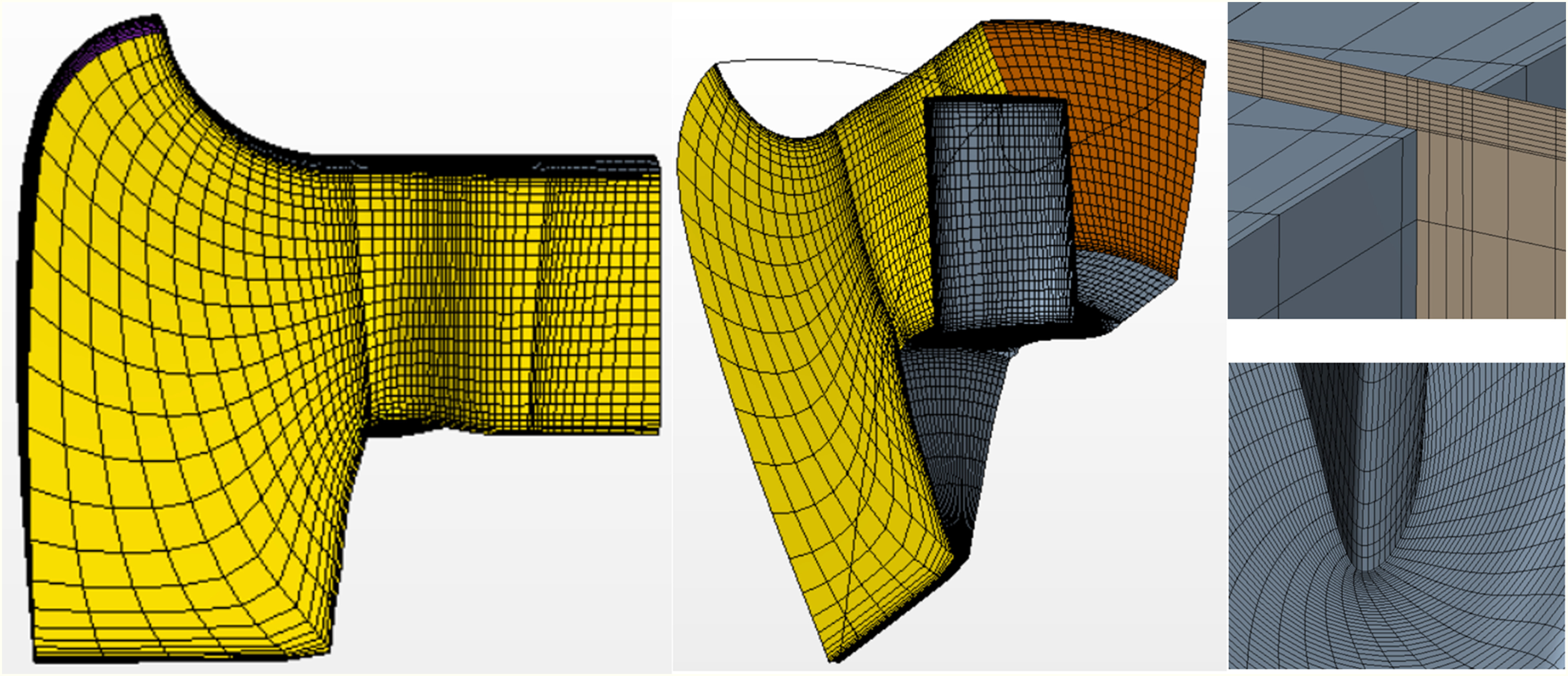
https://journal.gpps.global/f/fulltexts/204815/JGPPS-00263-2024-01.03_min.jpg

The brown-coloured section visible in the top-right frame of Figure 3 shows that blade tip gap includes 10 cell layers (with tc = 0.4%B when not differently specified). The near-wall grid refinement permits achieving y+ values below 10, 2, and 25 in most part of the blade, casing, and hub surfaces, respectively. The purple-coloured surface grid visible in the left-side frame of Figure 3 indicates the bell-mouth entrance surface in which the stagnation inlet has been imposed as boundary condition. The static pressure condition with radial equilibrium and target mass flow rate constraints was applied at the domain exit, whose surface grid is orange-coloured in the middle frame of Figure 3. The two yellow-coloured surfaces visible in the left and middle frames of Figure 3 indicate the conformal surface grids where the periodic boundary condition was imposed. Finally, the grey-coloured surfaces visible in all Figure 3 frames indicate solid walls, treated as no-slip surfaces with fixed rotational speed relative to the rotating reference frame used for the computation. In particular, the casing wall and the hub prolongation downstream of the rotor exit feature rotational speed opposite to the rotor speed (2,750 rpm) in the relative reference frame while all the other surfaces feature zero rotational speed relative to the computation reference frame.

Experimental setup

The experimental campaign was performed in the Thermal and Aeraulic Machines Laboratory of the Department of Industrial Engineering at the University of Padova, where an ISO5801 type-A test rig is available. The test rig (see the left frame of Figure 4) and related instrumentation were continuously improved during the years as well documented in several publication. Present measurements exploited exactly the same apparatus already employed in (Masi et al., 2022b), where it was stated that the measurements accuracy at best efficiency operation is not worse than 1.3%, 1%, and 2% for q_v, Δp, and η_aer data, in that order. The detailed description of the rig and instrumentation is available in (Masi et al., 2022b) and therein-referenced earlier publications by the same authors.

Figure 4.

Experimental setup: ISO 5801 type A test rig available in the lab at the University of Padova (left); detail of the CS fan blade mounting (middle); complete rotor and CS fan (right).

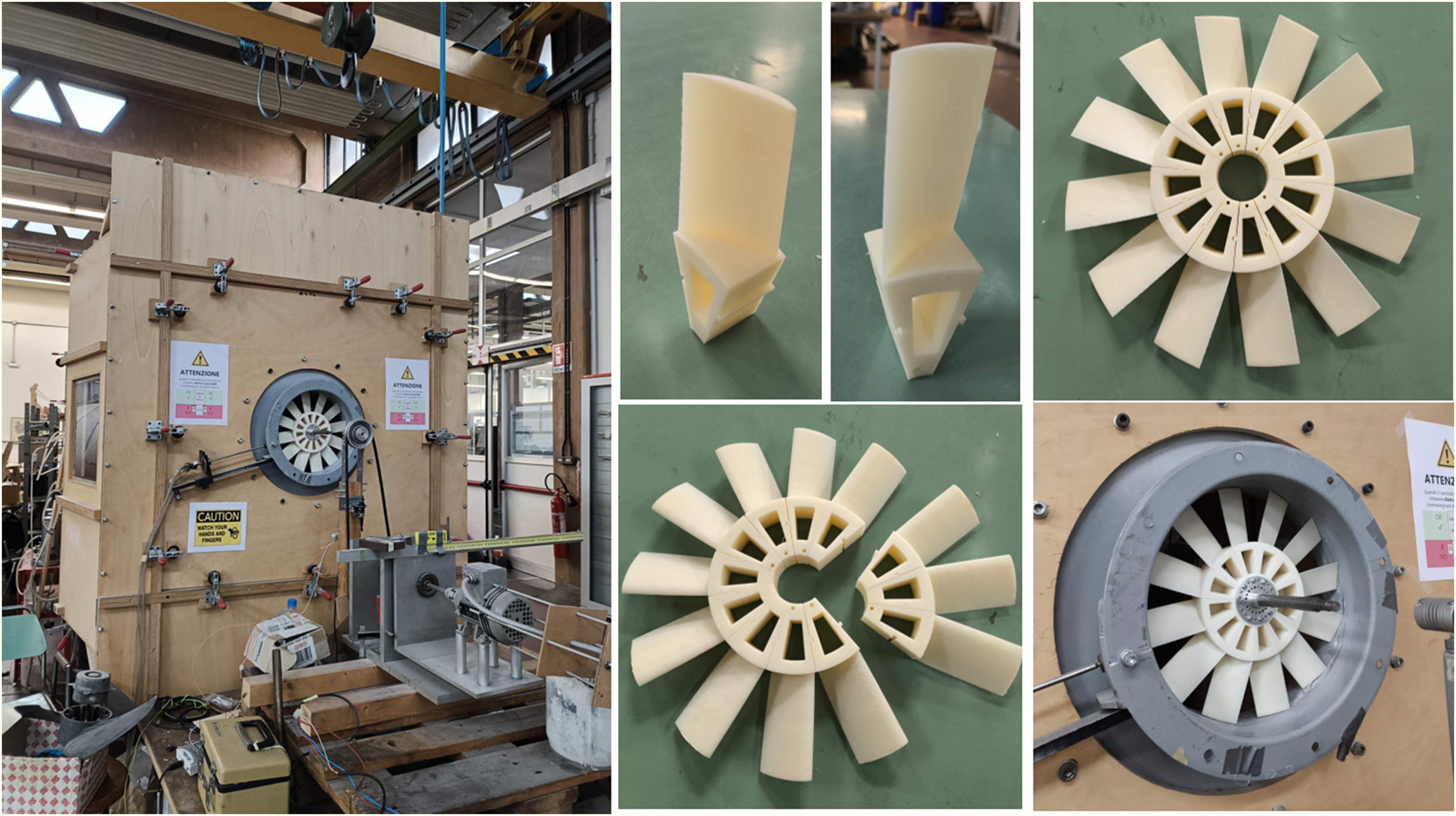
https://journal.gpps.global/f/fulltexts/204815/JGPPS-00263-2024-01.04_min.jpg

Aerodynamic global performance data were collected for the CS fan design, the rotor of which was manufactured in ABS by a rapid prototyping 3D printer in the size appropriate for the mounting on a 315 mm inner diameter casing taken from a commercial industrial fan. The two middle frames of Figure 4 refer to the details of the rotor mounting (where the strategy adopted for the blade assembling clearly emerges), whereas the two right frames show the complete CS rotor and the CS fan mounted on the rig, respectively.

Numerical validation of the fan designs

The CFD model described in the previous section was preliminarily used to validate the effectiveness of the adopted design methods in achieving the prescribed blade loading distribution. To this end, a simulation of the operation at Φ_d = 0.075 has been performed for each fan design in order to extract from the results the velocity distributions downstream of the rotor and compare them with the corresponding distributions expected by design.

Markers in Figure 5 show the ε_S (green), ε_A (red), and ε_R (blue) distributions predicted by CFD for each fan design at each computational cell intersected by a reference plane section perpendicular to the rotor axis, located 0.01D downstream of the blade root trailing edge. In particular, the top, middle, and bottom frames of the figure refer to the FV, RB, and CS designs in that order. Solid lines indicate the ε_S(x), ε_A(x), and ε_R(x), dimensionless velocity distributions expected by design, using the same colour convention as markers.

Figure 5.

Tangential (green), radial (blue), and axial (red) velocity ratios profiles at Φ_d = 0.075, as fixed by design (solid lines), and calculated by CFD (markers) 0.01D downstream of the blade root trailing edge for the FV (top), RB (middle), and CS (bottom) fan designs.

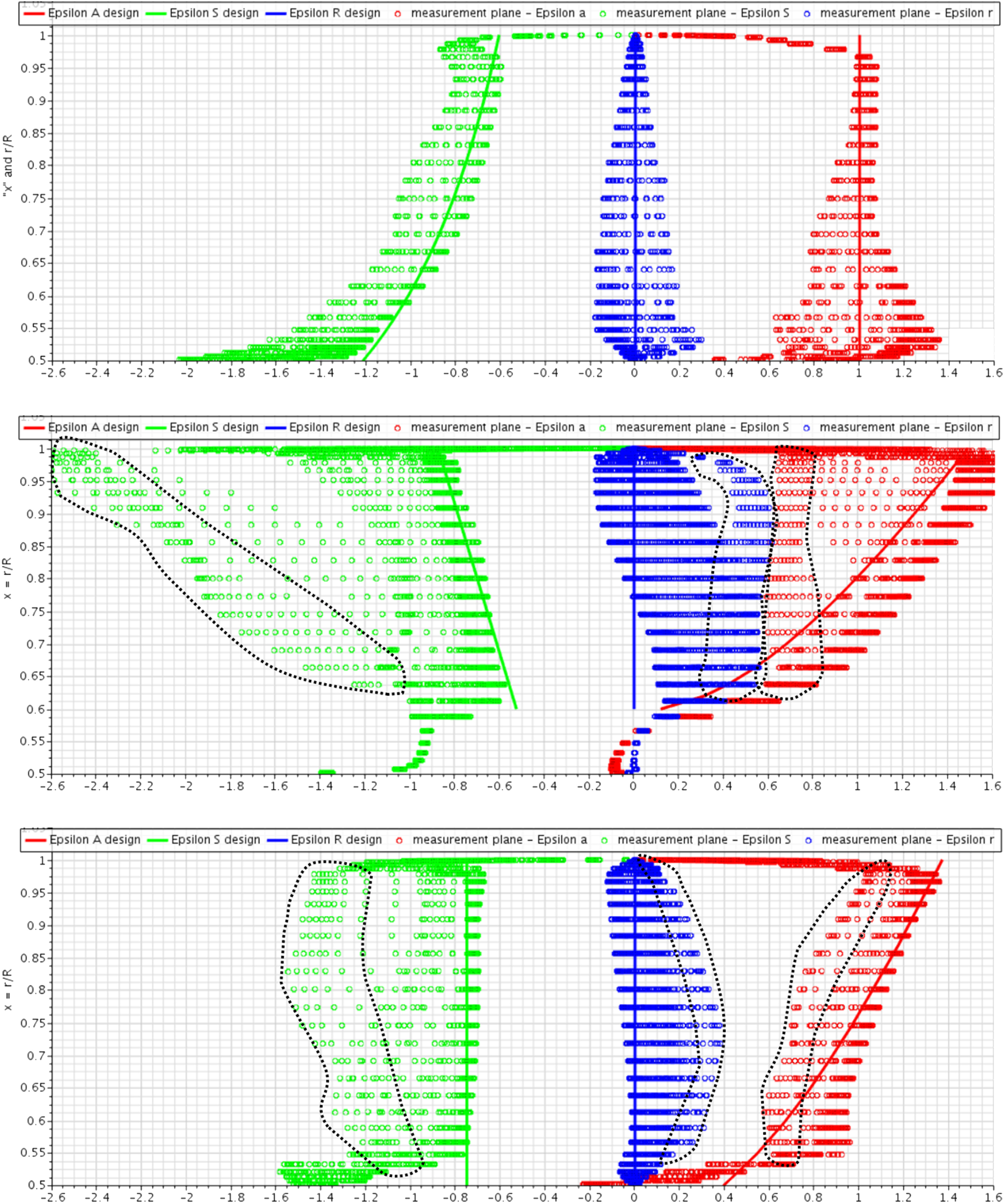
https://journal.gpps.global/f/fulltexts/204815/JGPPS-00263-2024-01.05_min.jpg

As a general observation, the average trends of marker clouds fairly approximate the design expectations, although the amplitude of markers scattering strongly depends on the fan design. Among the marker clouds of the three fans, those belonging to the FV design show the lower scattering and better agreement with distributions expected by design, followed by CS and RB designs in that order. The scattering trend is mainly affected by the space required to approach the radial equilibrium of the flow downstream of the rotor exit and by the distance of the reference plane from the average position of the blade trailing edge. The first is a minimum for the FV blade loading distribution and a maximum for the RB blade loading – due to the maximum uniformity of the specific work exchange and axial velocity component of the former, and the maximum radial velocity component locally arising from the latter. The second increases moving from RB to CS to FV – because of the different chord length at the blade root and different blade taper and twist associated with the three designs – and leaves the minimum and maximum space available to the RB and FV designs, respectively, for achieving radial equilibrium. Focusing on the agreement between average dimensionless velocity distributions predicted by CFD and expected by design, the differences among the three designs are mostly due to the different level of azimuthal flow uniformity achieved at the reference plane section. As already noted for the radial equilibrium condition, the limited scattering of CFD markers for the FV fan – if compared to the CS design and, even more, the RB design – is compatible with the azimuthal mixing of the blade wake and main throughflow which is almost completed only in the FV fan case. Especially for the RB design case, but also for the CS design, the scattering of each dimensionless velocity distribution show two accumulation curves, one resembling the trend expected by design, and one reproducing a very different trend. The latter has been enclosed by black point curves in the middle and bottom frames of Figure 5 to underline a low-axial-velocity flow with higher radial and tangential velocity components. This is compatible with the wakes released from the RB and CS blade trailing edges, not yet well mixed with the main flow. In the light of these arguments, it is concluded that all the fans approximate the blade loading distribution expected by design with comparable accuracy and to a level deemed as acceptable for the purpose of this work.

With regard to the RB design, the good agreement between CFD predictions and expected distribution of ε_A(x) in the portion of span in which ε_S(x) was imposed by design, demonstrates that the design assumption of considering the air flow below ν_aero as a solid extension of the real hub is effective.

Finally, the satisfactory agreement between ε_A(x) predicted by CFD and expected by design for the CS fan at 0.95 < x < 0.6 suggests that the criterion here proposed to estimate Γ, and included as an upgrade of the ML method, works fairly well for this specific design case and deserves further investigations to verify its degree of general validity.

Results and discussion

Figure 6 compares the aerodynamic global performance as predicted by CFD for the three fan designs. For the sake of appropriate comparison, all the designs were modelled with tc/B = 0.4%, although the CS blade shape resulted from the tc/B = 1.7 assumption. Such very low tc/B value was assumed to obtain indication on the maximum performance achievable by the three designs when manufactured for large size industrial applications (D ≥ 630 mm) in operation at Re ≈ 10⁶. The characteristic curves are reported in dimensionless form relying on the performance parameters based either on p_f data (on the left – best suited to ducted-fan installations) or p_fs data (on the right – best suited to exhaust-fan installations).

Figure 6.

Aerodynamic global performance curves: Ψ (upper-left), η_aer (lower-left), Ψ_TS (upper-right), and η_TS (lower-right) vs Φ, as predicted by CFD for the FV (blue), RB (red), and CS (black) fans. Point lines intersection marks the design point and segment markers indicate η_aer expected by design.

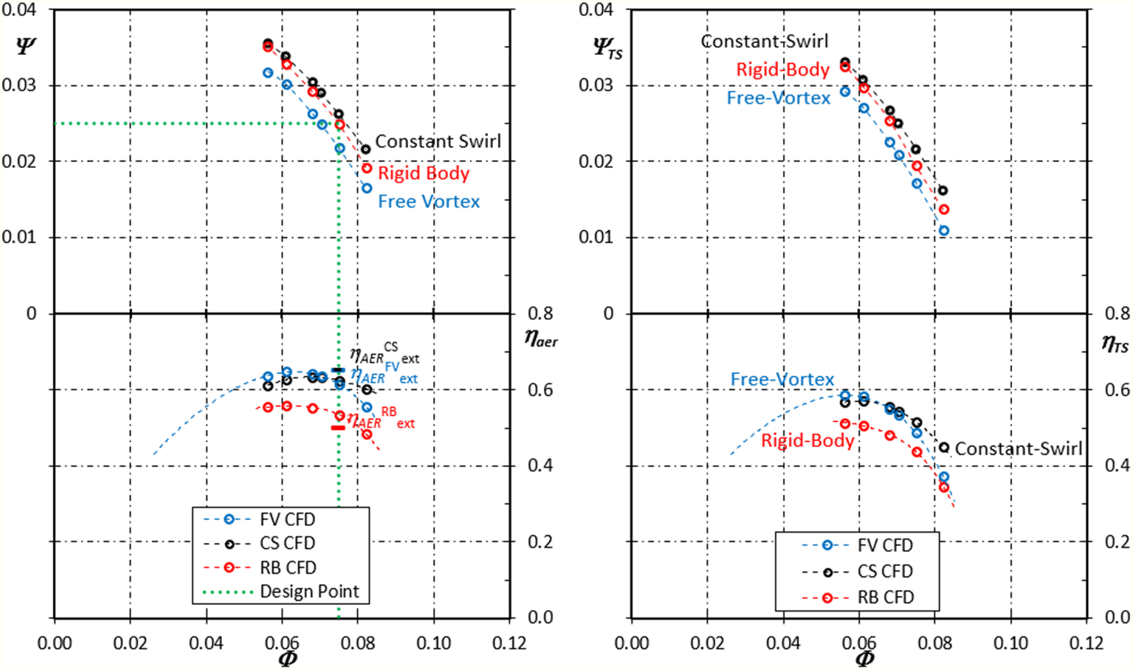
https://journal.gpps.global/f/fulltexts/204815/JGPPS-00263-2024-01.06_min.jpg

First of all, none of the three designs permits a perfect matching between Φ_d and the duty point where the maximum η_aer is achieved. However, the maximum difference in efficiency between these two operating conditions for the three fan designs never exceeds 2.5 percentage points, demonstrating that the employed methods are quite effective in designing fans with ν = 0.5.

Second, Ψ requirement at design is fulfilled by all designs except for FV (see the left-side-frame in Figure 6). Nevertheless, considering the higher Ψ predicted at peak η_aer operation for the FV fan, it is possible that also such design succeeds in the fulfilment of Ψ_d at Φ_d with η_aer comparable with the CS design. In fact, 2° to 3° adjustment of the blade position angle could allow achieving the duty point without strongly penalising the peak efficiency value, as for the case considered in (Masi et al., 2022b). Exactly because of the same argument, it is not expected that any blade positioning change could allow the RB design to approach the CS efficiency, whereas it is very likely RB design could exceed the CS design in terms of Ψ_d. Much the same observations hold in qualitative terms for the exhaust-installation case (right-side frames in Figure 6).

To quantify the quality of the FV, RB, and CS designs, their global performance are compared with those achieved by tube-axial fan design examples presented in the literature as the best possible solutions for Ω ≈ 4. In particular, (Bamberger and Carolus, 2015) simulated by experimentally validated CFD two 300 mm diameter fans in operation at 3,000 rpm, with exactly the same tc/B value as the one assumed here. The first fan – the BEM1 design – features ν = 0.55 and free-vortex blade loading, and it was designed by applying the boundary element preliminary design method reported in (Carolus and Starzmann, 2011). Its design point, referred to as DP2, is at Φ_d roughly 10% lower than the FV fan Φ_d, and 10% higher than Φ at which the FV fan operates at maximum η_aer. The second fan – the OPT fan, which features ν = 0.4 – is the result of the artificial-intelligence-driven optimisation process (already referenced in the Introduction) of the BEM1 design aimed at achieving the best possible η_TS. A first outcome of this comparison is that the BEM1 and FV fans, both resulting from application of classical preliminary design methods, achieve much the same aerodynamic performance, being Ψ_TS and η_TS equal to 0.0236 and 55.1% for the BEM1 fan and equal to 0.0225 and 55% for the FV fan. Accordingly, it can be stated that the FV design presented here is a state-of-the-art preliminary design with FV blade loading distribution. A second outcome of the comparison is that the OPT fan and the CS design achieve at OPT/BEM1 Φ_d operation much the same Ψ_TS (0.0265 the former and 0.0267 the latter) with η_TS equal to 59% and 55.6%, respectively. This means that the use of ML preliminary design method for applications with Ω ≈ 4.3 allows obtaining fan designs that match Ψ_TS achieved by designs already optimised, with η_TS approximately 3.5% lower than the value claimed as best possible, but 0.5% higher than η_TS achievable by application of classical preliminary design methods implementing the FV blade loading distribution.

In order to obtain information on the aerodynamic performance really achievable by the CS design when manufactured by using production technologies appropriate for the smaller sizes of real industrial applications and to search for a further validation of the CFD results, the CS fan was initially redesigned for tc/B = 0.8. In fact, such dimensionless value corresponds to an absolute tc in the order of 0.6 mm if applied to a 315 mm diameter fan. In the authors’ experience, this should have been the minimum tc/B value compatible with: (i) the slight eccentricity of the rotor shaft (due to the practical difficulty at the industrial level to assure a perfectly centred mounting of the electric motor on the supporting strut); (ii) the not perfect circularity of the fan casing inner surface; (iii) the mechanical vibrations associated with the not ideal balancing of the system. In fact, the prototype started working fine at reduced rotational speed but, during the ramp up to the design speed, the increased amplitude of vibrations, occurring when passing for a critical speed of the mechanical assembly, led to the failure of some blades due to excess of rubbing with the casing wall. Thus, the CS fan was finally designed, manufactured, and experimentally tested at 2,750 rpm with a safe value of tc/B equal to 1.7%, as previously reported in the Constant-swirl design Sub-section. Figure 7 reports the experimental data measured for the CS fan and compares them with the CFD results obtained for the same design with smaller tc/B values (black markers), and for the FV design with tc/B = 0.4 (blue markers).

Figure 7.

Aerodynamic global performance curves: total pressure coefficient (upper left), aeraulic efficiency (lower left), total-to-static pressure coefficient (upper right), and total-to-static efficiency (lower right) vs flow rate coefficient for the CS fan (black) as measured with 1.7% tc/B and predicted by CFD with 0.4% (circle markers) and 0.8% (diamond markers) tc/B, and for the fan FV (blue) as predicted by CFD with 0.4% (circle markers). Point lines intersection marks the design point.

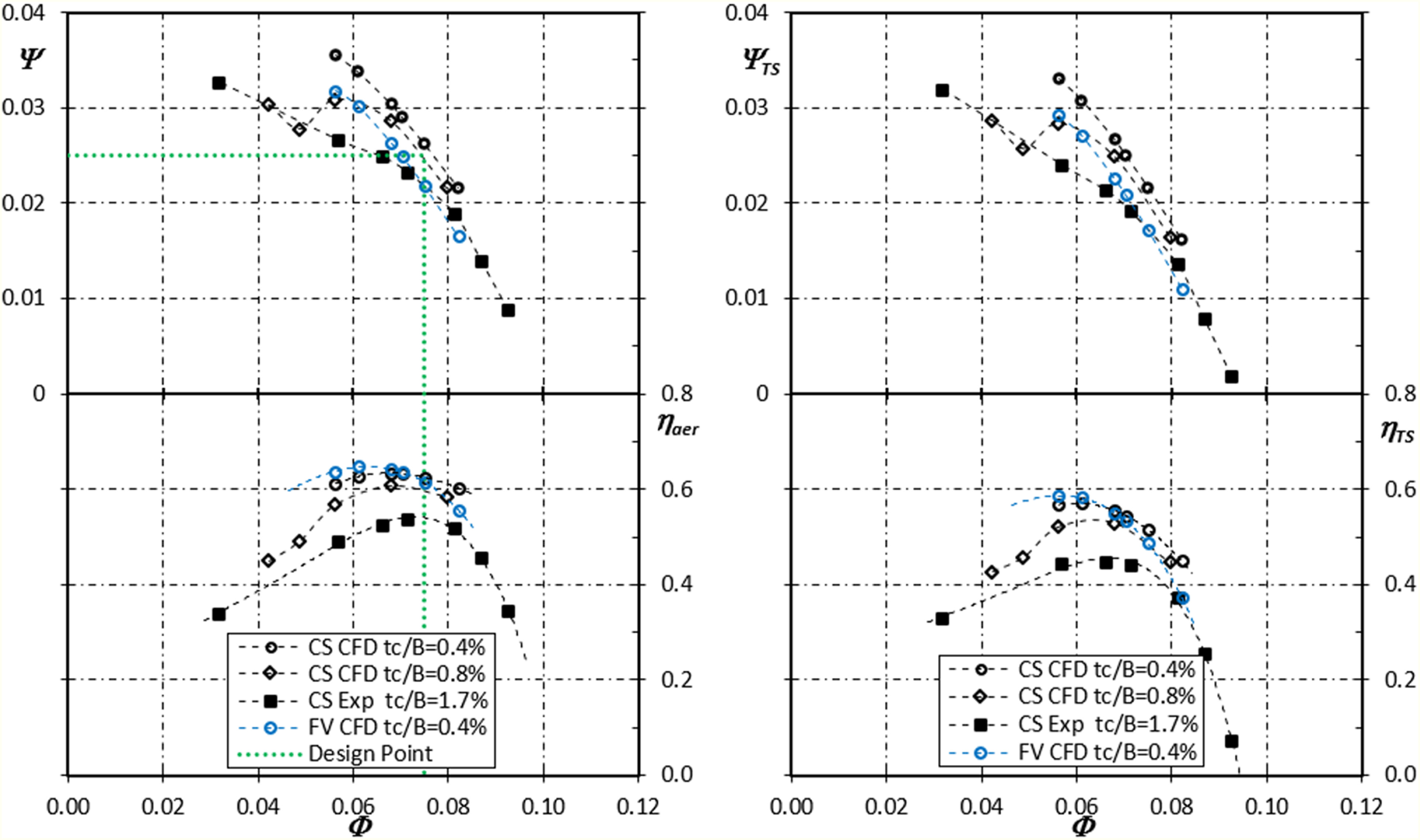
https://journal.gpps.global/f/fulltexts/204815/JGPPS-00263-2024-01.07_min.jpg

The decrease of both fan pressure and efficiency values as the tip gap increases is evident and compatible with the quantitative findings reported in (Downie et al., 1993). This is an indirect experimental validation of the CFD model numerically validated in Appendix B.

The experimental results underline the relatively high-pressure capability of the CS design, which is still able to match the FV design point operation even if manufactured with 4 times higher tc, although the corresponding efficiency decrease is very important. On the other hand, the CFD results indicate that when tc of the CS design is two times the tc of the FV design, the CS fan is still able to fulfil the original design requirement (not matched by the FV fan) with Ψ_TS higher than the FV fan and much the same η_aer and η_TS.

Conclusions

The preliminary design methods used to obtain three tube-axial fans with specific speed equal to approximately 4.3 and differing to each other for the sole blade loading distribution demonstrated that:

The ML method proposed some years ago by the authors to design fans with low hub-to-tip ratio and constant swirl blade loading, and later on satisfactorily applied in the hub-to-tip range from 0.2 to 0.4, is effective also for tube-axial fans with hub-to-tip equal to 0.5.
The use of the ML method to design fans implementing the constant-swirl blade loading is as effective as the use of the consolidated “Kahane-Wallis” method is to design fans implementing either the free-vortex or the rigid-body blade loading concepts.

The two modifications introduced to the ML method here for the first time, i.e., the new empirical criterion to estimate the obliquity of the meridional flow as a function of the tip gap, and the use of chart taken from the literature to assign the local aerofoil incidence, demonstrated that the revised ML method:

Is effective for the design of 0.5 hub-to-tip ratio fans that achieve the maximum efficiency in proximity of the desired design point, notwithstanding the removal of the constant local aerofoil incidence assumption which was basis of the previous version of the method.
Improves its level of general reliability owing to the elimination of arbitrary assumptions derived from experience, that were required for the application of the former version of the method.

The comparison of the global aerodynamic performance predicted by CFD for the fan designs implementing the free-vortex (FV), rigid-body (RB), and constat-swirl (CS) blade loading distributions demonstrated that:

The CS and RB blades are both able to fulfil the aerodynamic requirements of a 4.3 specific speed design with hub-to-tip equal to 0.5, but the latter at cost of approximately 15% lower efficiency than the former. Such efficiency penalty suffered by the RB design is associated with the strong concentration of the work exchange this blade loading concept imposes in the outermost part of the blade, which makes unavoidable the onset of a large flow separation at the blade root. The present results suggest that RB designs can be more attractive than CS design for specific speeds either appreciably lower than 4.3 (where the hub-to-tip ratios are higher) or appreciably higher than 4.3 (where the pressure requirements are lower).
The CS and FV blades achieve much the same efficiency, but the latter at cost of approximately 15% lower fan pressure than the former. Such fan pressure penalty suffered by the FV design is associated with the excessive concentration of the aerodynamic load this blade loading concept imposes in the innermost part of the blade. This leaves largely under-exploited most of the blade span to avoid lift coefficients at the blade root unacceptably high for efficiency and stall margin. However, there are designs documented in the literature that are claimed to implement a roughly-FV blade loading distribution defined by optimisation techniques which permit exceeding the fan pressure and efficiency levels of the FV design presented here. This suggests that the optimal blade loading for specific speeds in the around of 4.3 could ideally lay in between the FV and CS blade loading concepts.

On the other hand, the CFD results integrated by the experimental data presented here, demonstrated that the CS design outperforms the FV design if the tip gap cannot be reduced down to less than 0.5% of the blade height – as for the case of small size tube-axial industrial fans – where a CS design with a reasonable dimensionless tip gap (0.8%) permits fan pressure 8% higher than a FV design with an hard-to-manufacture dimensionless gap (0.4%), at much the same efficiency level.

Although the findings of this work lack of general validity, being related to a specific design case, they were obtained owing to the definition of a general framework that allows to study all cases deemed as necessary to integrate the information already available from the literature and arrive to conclusions valid for the design of the whole tube-axial fans type.

Nomenclature

ANN

artificial neural network

AR = B/l

blade aspect ratio, based on l at midspan (−)

blade height, (m)

C_D = C_Dp

aerofoil (profile) drag coefficient, (−)

C_Ds, C_Dew

secondary and end-wall loss coefficients, (−)

C_L

aerofoil lift coefficient, (−)

fan diameter, (m)

CFD

computational-fluid-dynamics

constant swirl blade loading distribution

free vortex blade loading distribution

K_i

mutual interference factor – rectilinear 2D cascade to isolated aerofoil lift coefficients ratio, (−)

Kahane-Wallis

Masi-Lazzaretto

mechanical power at rotor shaft, (W)

RANS

Reynolds averaged Navier-Stokes

rigid body blade loading distribution

ca¯

mean axial velocity in the annulus, (m/s)

c_a, c_r, c_u

local axial, radial, and tangential velocity components at rotor exit, (m/s)

nose droop – extra-camber addition at aerofoil leading edge, (m)

aerofoil chord, (m)

pressure, (Pa)

p_f

fan pressure (ISO 5801), (Pa)

p_fs

total-to-static pressure rise (ISO 5801), (Pa)

q_v

fan volumetric flow rate, (m³/s)

radial coordinate, (m)

aerofoil maximum thickness, (m)

tip clearance, (m)

x = r/r_tip

dimensionless radial coordinate, (−)

x₀

x coordinate of rotor exit plane points where the radial equilibrium condition fixes ca(x0)=ca¯, (−)

rotor blade counts, (−)

Greeks

attack angle – angle between local mean relative velocity and aerofoil chord, (°)

β₁

relative flow angle at rotor entrance– angle between local relative velocity and rotor axis, (°)

β_m

mean relative flow angle – angle between local mean relative velocity and rotor axis, (°)

meridional flow obliquity – angle between local meridional velocity and rotor axis, (°)

εA=ca/ca¯

local axial velocity ratio at rotor blade exit, (−)

εR=cr/ca¯

local radial velocity coefficient at rotor blade exit, (−)

εS=cu/ca¯

local swirl coefficient at rotor blade exit, (−)

η_aer = q_v p_f /P

fan aeraulic efficiency (ISO 5801), (−)

η_loc

local blade aerodynamic efficiency, (−)

η_TS = q_v p_fs /P

fan total-to-static efficiency, (−)

aerofoil camber – angle between meanline tangents at the aerofoil leading and trailing edges, (°)

local incidence – angle between relative velocity and aerofoil camber line at the rotor entrance, (°)

hub-to-tip ratio, (−)

ν_aero

“aerodynamic” hub-to-tip ratio (innermost dimensionless radius considered for blade design), (−)

air ass density, (kg/m³)

σ = lz/(2π r)

local blade solidity, (−)

stagger angle – local angle between aerofoil chord and rotor axis, (°)

ϕ_P

blade position angle – local angle between aerofoil chord and rotor plane, (°)

angular velocity, (rad/s)

mean obliquity of the meridional flow within the blade passage, (°)

Δ = Ψ_d^0.25/Φ_d^0.5

specific diameter (−)

ΔH = Δp/ρ

increase of mechanical energy per unit mass (J/kg)

Φ = q_v/(ωD³)

fan flow rate coefficient, (−)

Ψ = p_f /ρ/(ωD)²

fan total pressure coefficient, (−)

Ψ_TS = p_fs/ρ/(ωD)²

fan total-to-static pressure coefficient, (−)

Ω = Φ_d^0.5/Ψ_d^0.75

specific speed (−)

Subscripts

design

_{ext, is}

expected, isentropic

_{hub, tip, casing}

hub, tip, casing

Appendix A – Main steps of the design processes

All blade design methods perform the three major design steps reported in the following as rearrangement of what indicated in the well-known KW method, originally suggested by (Kahane, 1948) – for blade designs strongly departing from FV blade loading – and successively evolved by (Wallis, 1993), up to its definite formalisation presented in (Downie et al., 1993).

Definition of the velocity diagrams that fulfil the fan aerodynamic performance requirements. This design step starts with the assumption of the spanwise distributions for ε_S and blade aerodynamic efficiency (η_loc), as well as a reasonable value for η_aer of the fan. The solution of the radial equilibrium equation at the rotor exit under the continuity constraint allows determining the unknown ε_A(x) distribution. The global isentropic pressure coefficient can be therefore calculated through mass-flow-weighted integration along the whole blade span, as reported in Equation A1.
( \rm A1)
Ψis=∫ν1⁡[xεS(x)2πΦd(1−ν2)εA(x)]xdx∫ν1⁡εA(x)xdx
Finally, η_aer allows for assessing the achievement of the desired fan pressure coefficient at design (Ψ_d). This design step needs for completion very few iterations, in which the initial assumption of ε_S(x) is progressively adjusted up to the desired Ψ_d is achieved. The availability of the dimensionless coefficients in Equation 3 make available the corresponding spanwise distributions of the velocity diagrams and related mean relative flow angle (β_m).
Individuation of the aerofoil sections that makes possible the work exchange associated with the velocity diagrams. The set of aerofoil sections defining the skeleton of the rotor blade must fulfil Equation A2, where the dependency of all parameters on x has been omitted for the ease of reading. In particular, Equation A2 states that each aerofoil section – once stacked at the appropriate x and azimuthally replicated in an annular cascade with local solidity equal to σ – shall assure aerodynamic performance (read, C_L, C_Dp, C_Ds, and C_Dew) that permits obtaining the local velocity diagrams (read, ε_S, ε_A, and β_m).
( \rm A2)
σCL(α)Ki(σ,ξ(βm,α))=2εScos⁡(βm)0.5(1+εA)−σ{CDp(CL(α),σ)+CDs(CL(α))+CDew(σ)}tan(βm)
Note that: i) the cascade loading factor (i.e., the Equation A2 left-hand-side) is affected by the mutual interference factor between adjacent aerofoils (K_i); ii) the secondary and end-wall losses are accounted for by charging each blade element with two additional local drag coefficients (C_Ds and C_Dew, respectively). Functional dependencies in Equation A2 show that from the analytical point of view, for a given aerofoil section, the selection of the attack angle (α) fixes the values of the aerodynamic coefficients and, accordingly, σ remains univocally defined.
Quantification of the blade stagger. The last design step is performed via Equation A3.
( \rm A3)
ξ(x)=βm(x)−α(x)

Since the value of the stagger angle (ξ), was already required in the previous design step, some iterations of steps 2 and 3 must be performed to complete the blade design.

Appendix B – Grid sensitivity study

The present authors tested the simulation approach used here on several tube-axial fan designs with different ν, and assessed its satisfactory capability to predict the global aerodynamic performance curves in the stable operation range of the fan. In particular, (Danieli et al., 2020) documented in detail the sensitivity of such simulation approach to grid size, streamwise extension of the fluid domain, and turbulence model. Moreover, the simulation approach was experimentally validated against the global performance and local velocity components at the rotor exit plane as measured for a tube-axial fan with ν = 0.28. However, the three fan designs subject of the present paper feature ν well in excess of 0.28. In addition, as shown in the left and middle frames of Figure 3, the flow domain considered here provides the real bell-mouth and hub shape at the rotor entrance. This was not the case of the models used in (Danieli et al., 2020) that assumed a fully-developed annular flow upstream of the rotor as for a fan installed in a long duct and equipped with an infinitely long hub. Due to these non-negligible differences, it was decided to repeat the grid sensitivity study for the FV fan at Φ = 0.0703 as representative of all the 3 fan designs, assuming that the final grid setup chosen for the FV fan assures comparable accuracy level when applied to both the CS and RB fan designs. To estimate the numerical uncertainty of the CFD results due to the discretisation error (not model errors), the values predicted for 4 global performance parameters by computations performed on 3 grids with different element counts have been considered by using the well-known procedure formalised by (Celik et al., 2008), based on the Richardson extrapolation method. The first column in Table B1 indicates the parameters needed to estimate the discretisation error using the same naming convention as that suggested in (Celik et al., 2008). The other 4 columns report the values obtained for each performance parameter (ϕ) taken into account (i.e., Ψ, Ψ_TS, η_aer, and η_TS in that order).

Table B1.

Calculation of discretisation for the CFD model applied to the FV fan design in operation at Φ = 0.0703.

	ϕ = Ψ	ϕ = Ψ_TS	ϕ = η_aer	ϕ = η_TS
N₁, N₂, N₃	244,702, 106,508, 36,896	244,702, 106,508, 36,896	244,702, 106,508, 36,896	244,702, 106,508, 36,896
r₂₁, r₃₂	1.32, 1.42	1.32, 1.42	1.32, 1.42	1.32, 1.42
ϕ₁,ϕ₂,ϕ₃	0.02498, 0.02493, 0.02506	0.02096, 0.02091, 0.02103	0.6357, 0.6364, 0.6359	0.5333, 0.5336, 0.5338
p	2.69 (oscillatory conv.)	2.58 (oscillatory conv.)	1.46 (oscillatory conv.)	2.77 (monotonic conv.)
ϕ²¹_ext	0.02503	0.02101	0.6343	0.5330
e²¹_a, e²¹_ext	0.21%, 0.19%	0.26%, 0.25%	0.11%, 0.22%	0.06%, 0.05%
GCI²¹_fine	0.24%	0.31%	0.28%	0.06%

Note that Table B1 data refer to computations performed on grids with the same cell layer counts in the blade tip gap (4 cells within a gap equal to 0.4% of the blade height), to assure an effective progressive refinement of the grid in the bulk-flow region. Remarkably, the results demonstrate that the coarse grid (N₃, which counts approximately 37,000 cells for a blade passage) is already capable of satisfactory accuracy as far as the fan global aerodynamic performance is concerned. This is not much surprising since such cell counts, if applied to one of the 12 blade passage of a 315 mm diameter rotor, correspond to a domain-average cell length approximately equal to 3 mm, which is well in excess of the local cell size in the rotor region. On the other hand, to evaluate the accuracy error due to the discretisation chosen for the tip gap region, two additional computations have been performed on the fine grid (N₁) with increased number of elements in the blade tip gap. Table B2 shows in columns 3 to 6 the values obtained for the global performance parameters and, in column 7, the tip gap flow rate (as fraction of the blade channel flow rate). Each line refers to a grid with a specific number of cell layers in the tip gap. For the sake of easier comparison, first line data repeat those already showed in Table B1 for the N₁ grid. It appears that neither the tip gap flow rate nor the fan global performance predictions change remarkably passing from 7 to 10 cell layers in the tip gap. This, added to the limited difference in fan performance predictions demonstrated by N₂ and N₁ grids, leads to select for the three fan design computations a final grid, whose cell counts and performance predictions are reported in the last line of the table.

Table B2.

Comparison between CFD predictions as a function of the tip gap grid refinement for the performance of the FV fan design in operation at Φ = 0.0703.

Grid ID/cell layers in the tip gap	Cell counts (overall)	Ψ	Ψ_TS	η_aer	η_TS	Tip leakage/channel flow rate (‰)
N₁/4	244,702	0.02498	0.02096	0.6357	0.5333	4.26
N₁/7	246,022	0.02504	0.02102	0.6363	0.5341	4.21
N₁/10	247,342	0.02497	0.02095	0.6343	0.5330	4.19
Final/10	187,846	0.02497	0.02095	0.6358	0.5334	4.11

FUNDING

No funding sources

COMPETING INTERESTS

Massimo Masi declares that he has no conflict of interest. Piero Danieli declares that he has no conflict of interest. Enrico Dal Cin declares that he has no conflict of interest. Edoardo Bregolin declares that he has no conflict of interest.

REFERENCES (29)

Angelini G., Corsini A., Delibra G., and Tieghi L. (2019). A multidimensional extension of Balje chart for axial flow turbomachinery using artificial intelligence-based meta-models. Journal of Engineering for Gas Turbines and Power. 141 (11): 4044935. 10.1115/1.4044935.

CrossRef

Google Scholar

Baljé O. E. (1981). Turbomachines – A Guide to Design, Selection, and Theory. New York: John Wiley & Sons.

Google Scholar

Bamberger K. and Carolus T. (2014). Performance prediction of axial fans by CFD-trained meta-models. In: Proc. ASME Turbo Expo 2014. GT2014-26877, V01AT10A028.

Google Scholar

Bamberger K. and Carolus T. (2015). Analysis of the flow field in optimized axial fans. In: Proc. ASME Turbo Expo 2015. GT2015-43205, V001T09A013.

Google Scholar

Bamberger K. and Carolus T. (2020). Efficiency limits of fans. Proceedings of the Institution of Mechanical Engineers, Part A: Journal of Power and Energy. 234 (5): 739–748. 10.1177/0957650919876838.

CrossRef

Google Scholar

Carolus T. and Starzmann R. (2011). An aerodynamic design methodology for low pressure axial fans with integrated airfoil polar prediction. In: Proc. ASME Turbo Expo 2011. GT2011-45243.

Google Scholar

Casey M. V. (1987). A mean-line prediction method for estimating the performance characteristic of an axial compressor stage. In: Proc. Inst. Mech. Eng.. Paper C264/87.

Google Scholar

Celik I. B., Ghia U., Roache P. J., Freitas C. J., Coleman H., and Raad P. E. (2008). Procedure for estimation and reporting of uncertainty due to discretization in CFD applications. Journal of Fluids Engineering. 130: 078001-1/4.

Google Scholar

Cordier O. (1953). Ähnlichkeitsbedingungen für Strömungsmaschinen. Brennstoff-Wärme-Kraft. 5 (10): 337–340.

Google Scholar

10.

Csanady G. T. (1964). Theory of Turbomachinery. Waterloo: McGraw-Hill.

Google Scholar

11.

Danieli P., Masi M., Delibra G., Corsini A., and Lazzaretto A. (2020). Assessment of MULTALL as computational fluid dynamics code for the analysis of tube-axial fans. Journal of Turbomachinery. 143: 071005-1/10.

Google Scholar

12.

Downie R. J., Thompson M. C., and Wallis R. A. (1993). An engineering approach to blade designs for low to medium pressure rise rotor-only axial fans. Experimental Thermal and Fluid Science. 6: 376–401. 10.1016/0894-1777(93)90016-C.

CrossRef

Google Scholar

13.

Eck B. (1973). Fans. Oxford: Pergamon Press.

Google Scholar

14.

Engineering Sciences Data Unit (1980). A guide to fan selection and performance. ESDU 79037.

Google Scholar

15.

Hay N., Metcalfe R., and Reizes J. A. (1978). Simple method for the selection of axial fan blade profiles. Proceedings of the Institution of Mechanical Engineers, Part A: Journal of Power and Energy. 192: 269–275.

Google Scholar

16.

Kahane A. (1948). Investigation of axial-flow fan and compressor rotors designed for three-dimensional flow. In: National Advisory Committee for Aeronautics. Langley Aeronautical Lab. NACA TN-1652.

Google Scholar

17.

Lewis R. I. (1996.) Turbomachinery Performance Analysis. London: Arnold.

Google Scholar

18.

Masi M. and Lazzaretto A. (2019a). A new practical approach to the design of industrial axial fans: tube-axial fans with very low hub-to-tip ratio. Journal of Engineering for Gas Turbines and Power. 141: 101003-1/10. 10.1115/1.4044206.

CrossRef

Google Scholar

19.

Masi M. and Lazzaretto A. (2019b). A new approach to the design of industrial axial fans. Part II: forward-swept blades with low hub-to-tip ratio. In: Proc. ASME Turbo Expo 2019. GT2019-91532, V001T09A008.

Google Scholar

20.

Masi M. and Lazzaretto A. (2021). The design of tube-axial fans with forward inclined blades (in Italian). In: La Termotecnica, Anno LXXV, marzo 2021. pp. 68–73.

Google Scholar

21.

Masi M., Piva M., and Lazzaretto A. (2014). Design guidelines to increase the performance of a rotor-only axial fan with constant-swirl blading. In: Proc. ASME Turbo Expo 2014. GT2014-27176, V01AT10A033.

Google Scholar

22.

Masi M., Danieli P., and Lazzaretto A. (2022a). Overview of the best 2020 axial-flow fan data and inclusion in similarity charts for the search of the best design. Journal of Turbomachinery. 144 (9): 0901012. 10.1115/1.4053535.

CrossRef

Google Scholar

23.

Masi M., Lazzaretto A., Danieli P., and Bettanini C. (2022b). Design of a small axial-flow fan with 0.2 hub-to-tip ratio. In: Proc. International conference on fan noise, aerodynamics, applications and systems - FAN 2022. Paper 045.

Google Scholar

24.

Smith S. F. (1965). A simple correlation of turbine efficiency. The Journal of the Royal Aeronautical Society. 69: 467–470.

Google Scholar

25.

Smyth J. M. and Miller R. J. (2021). Selecting a compressor meridional topology: axial, mixed, radial. In: Proc. ASME Turbo Expo 2021. GT2021-59121, V02CT34A013.

Google Scholar

26.

Wallis R. A. (1968). A rationalised approach to blade element design, axial flow fans. In: Proc 3rd Australasian Conference on Hydraulics and Fluid Mechanics. Paper 2599.

Google Scholar

27.

Wallis R. A. (1993.) Axial Flow Fans and Ducts. Reprint. Malabar: Krieger.

Google Scholar

28.

Wang J. and Kruyt N. P. (2020). Validation of CFD simulations of aerodynamic performance of low-speed axial fans with low hub-to-tip ratio. In: Proc AIAA Scitech 2020 Forum. Paper 0345.

Google Scholar

29.

Wang J. and Kruyt N. P. (2022). Design for high efficiency of low-pressure axial fans with small hub-to-tip diameter ratio by the vortex distribution method. Journal of Fluids Engineering. 144 (8): 081201. 10.1115/1.4053555.

Journal Issues

Indexes

Table of contents

Introduction Methodology Numerical and experimental tools Numerical validation of the fan designs Results and discussion Conclusions Nomenclature Appendix A – Main steps of the design processes Appendix B – Grid sensitivity study FUNDING COMPETING INTERESTS REFERENCES

Introduction

Conceptual design

(1)

(2)

Basic sizing of the blade

Recent findings on tube-axial fan preliminary design

General fan research gap

Authors’ fan research gap

Aims of the work

Structure of the paper

Novelty and originality

Methodology

Figure 1.

Sketch of a tube-axial fan meridional view with the main geometrical parameters and the local velocity triangles in dimensional (left) and dimensionless (right) form.

(3)

Free-vortex design

(4)

(5)

Figure 2.

Perspective views of the FV (left), RB (middle), and CS (right) fan designs.

Rigid-body design

(6)

(7)

(8)

Constant-swirl design

(9)

(10)

(11)

(12)

(13)

Numerical and experimental tools

CFD model

Figure 3.

Surface grid of the computational domain: meridional view (left); perspective view (middle); detail of the blade surface grid and a meridional section of the volume mesh in the tip gap region (upper right); detail of the blade leading edge surface grid close to the hub (lower right).

Experimental setup

Figure 4.

Experimental setup: ISO 5801 type A test rig available in the lab at the University of Padova (left); detail of the CS fan blade mounting (middle); complete rotor and CS fan (right).

Numerical validation of the fan designs

Figure 5.

Tangential (green), radial (blue), and axial (red) velocity ratios profiles at Φd = 0.075, as fixed by design (solid lines), and calculated by CFD (markers) 0.01D downstream of the blade root trailing edge for the FV (top), RB (middle), and CS (bottom) fan designs.

Results and discussion

Figure 6.

Aerodynamic global performance curves: Ψ (upper-left), ηaer (lower-left), ΨTS (upper-right), and ηTS (lower-right) vs Φ, as predicted by CFD for the FV (blue), RB (red), and CS (black) fans. Point lines intersection marks the design point and segment markers indicate ηaer expected by design.

Figure 7.

Conclusions

Nomenclature

Greeks

Subscripts

Appendix A – Main steps of the design processes

( \rm A1)

( \rm A2)

( \rm A3)

Appendix B – Grid sensitivity study

Table B1.

Calculation of discretisation for the CFD model applied to the FV fan design in operation at Φ = 0.0703.

Table B2.

Comparison between CFD predictions as a function of the tip gap grid refinement for the performance of the FV fan design in operation at Φ = 0.0703.

Tangential (green), radial (blue), and axial (red) velocity ratios profiles at Φ_d = 0.075, as fixed by design (solid lines), and calculated by CFD (markers) 0.01D downstream of the blade root trailing edge for the FV (top), RB (middle), and CS (bottom) fan designs.