Test rig configuration

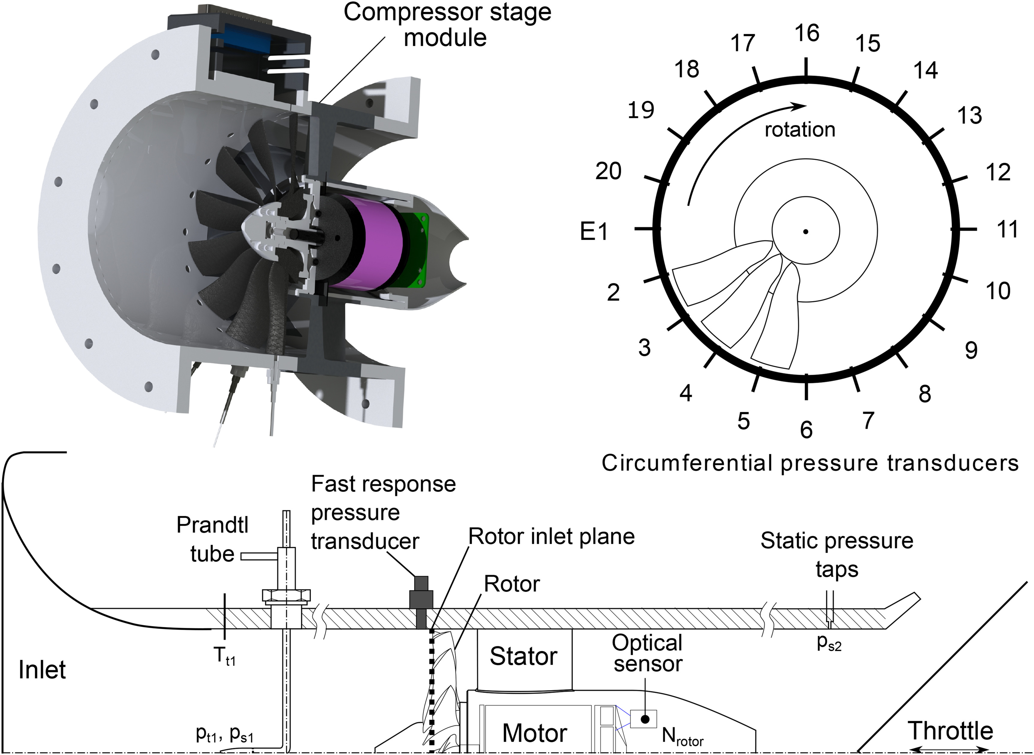
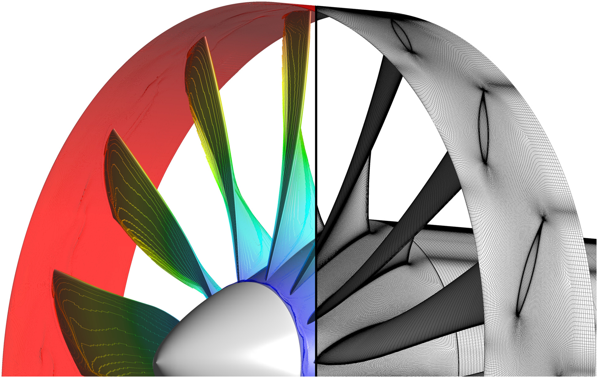
The low-speed axial compressor at the Chair of Aero Engines in the Technische Universität Berlin is employed for the transient throttling experiments. The stage consists of 14 composite carbon fiber blades based on the NACA-65 Profile and eight aluminum-printed stator vanes (see Figure 1). The open-flow wind tunnel is equipped with an adjustable throttle cone to regulate the mass flow for each operating point (OP) on the speed line. Two distinct tip clearance sizes have been produced by using different sets of blades. 15 flush-mounted pressure taps are evenly distributed at equidistant intervals downstream the stator. To further enable the spectral analysis of the throttling data, 20 fast-response pressure transducers were flush mounted to the casing wall with an axial offset of 1 mm upstream of the rotor inlet plane. The rotational speed for all OPs is 10,000min-1, with a sampling rate of 56 kHz. For each OP with constant throttling, the measurement time was 30 s or 5,000 revolutions. For the transient throttling runs, ca. 11 s or 1,800 revolutions were considered.

Figure 1.

Selected instrumentation features in the single-stage axial compressor at the Chair for Aero Engines, Technische Universität Berlin.

Speedlines and spectral behavior

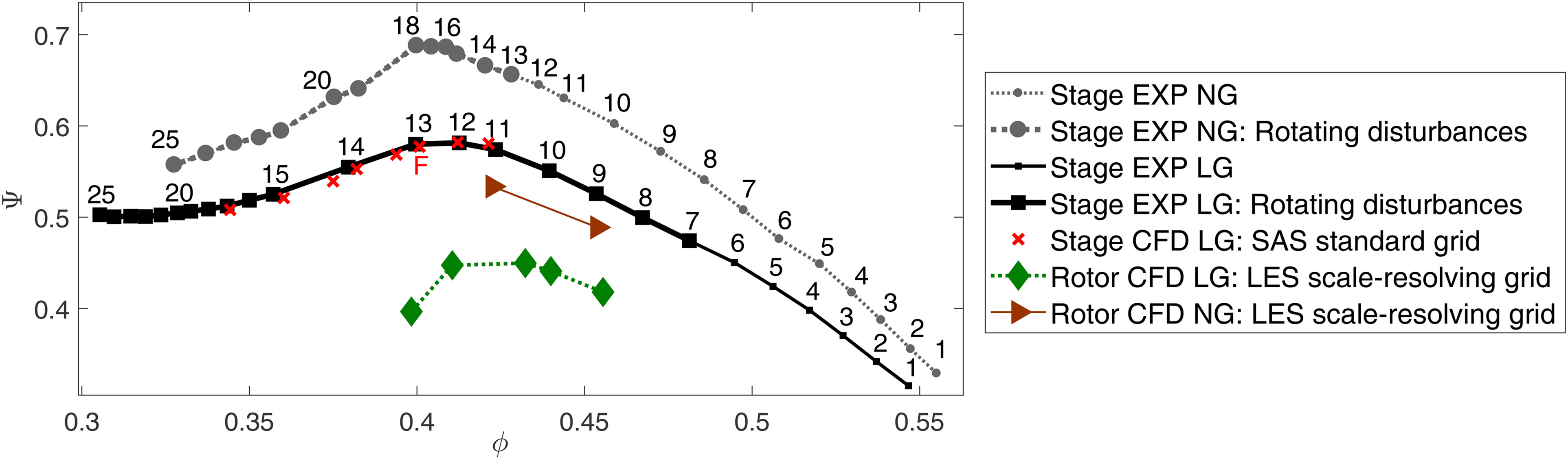
Before focusing on transient throttling investigations, it is insightful to refer back to typical speedlines, where the upstream and downstream boundary conditions are kept constant for each run. Performance results for these classic speedlines are shown in Figure 2 for both experimental runs considering the whole stage and selected simulations. Both the nominal gap (NG) and large gap (LG) configurations are displayed. The flow coefficient is defined as ϕ=cm1/umid and the total-to-static pressure rise as ψ=(ps2−pt1)/(0.5ρumid2). Here, umid is the blade velocity at mid-span and cm1 the inlet velocity. OPs for the experimental runs go from 1 (high mass flow) to 25 (low mass flow). The labeling is consistent with previous work (see de Almeida et al., 2024).

Figure 2.

Performance results for experimental (EXP) and unsteady simulations (CFD) of test rig at the TU Berlin. NG: nominal gap; LG: large gap. Rotor-only and stage setups are indicated, including the regions where rotating disturbances were experimentally detected. All CFD runs are full-annulus unsteady, both for the standard and the scale-resolving grids. SAS: Scale-Adaptive Simulation; LES: Large Eddy Simulation.

Focusing on the experimental speedline, the pressure spectrum of the flush-mounted probes on the rotor casing (refer to Figure 1) is shown in Figure 3 for both clearance setups. The horizontal axis is normalized by the blade passing frequency (BPF). Vertical doted lines indicate engine orders (EO), with evident local peaks. These peaks are not performance or fluid dynamic relevant and are linked to inherent geometrical irregularities. To minimize their presence, a straightforward technique was employed a priori for each of the fast-response pressure sensors: (i) the signal was shifted in time with the pitch offset to the neighboring probe, so that their phase match; (ii) one signal is subtracted from the neighboring probe’s signal and finally (iii) the spectrum was individually computed. With this approach, the amplitudes are obviously reduced, but the spectrum now shows the physical phenomena clearer. The spectra shown in Figure 3 are the average of all pressure transducers after this procedure was carried out.

Figure 3.

For different rotor clearances, the experimental spectrum from case-mounted pressure probes for operating points in Figure 2 is shown. The frequency is normalized by the blade passing (BPF). Engine orders shown by dashed vertical lines. (a) Nominal gap and (b) Large gap.

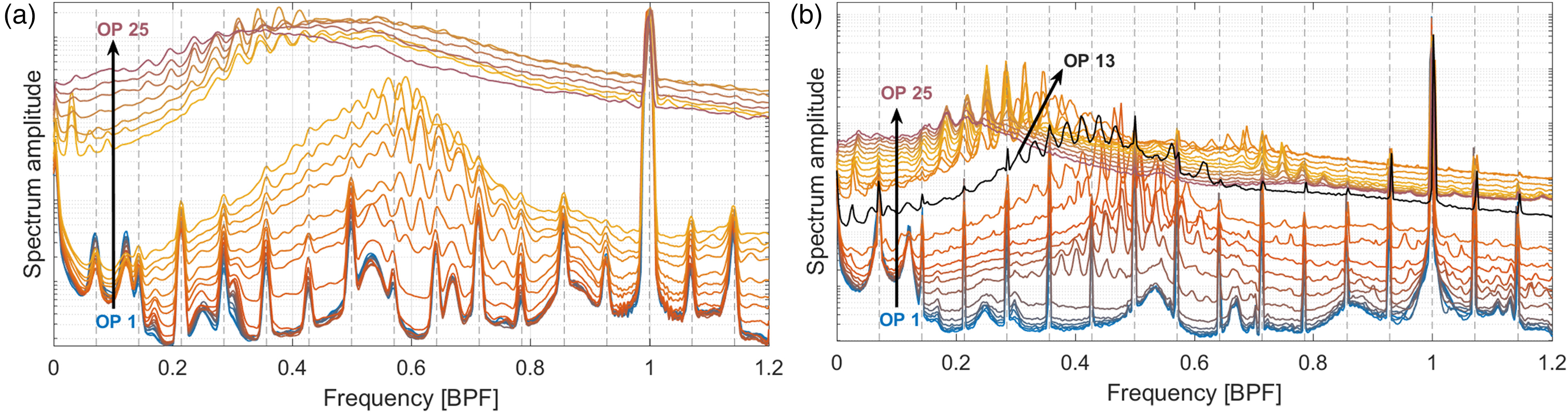
The region where rotating disturbances were experimentally detected is depicted in Figure 2 for both clearance configurations. It starts at OP 13 and OP 7 for the NG and LG setups respectively. This can be confirmed with the spectral curves from Figure 3, which show the typical prestall disturbance equidistant peaks around half the BPF. The onset of these prestall disturbances occurs with higher throttling but still before distinct flow separation. Part-span stall itself takes place past the peak of the characteristic (OP 18 for NG and OP 13 for LG). For lower flow coefficients, a clear increase in the pressure fluctuation is observed (one order of magnitude), as well as a shift in the peaks towards lower frequencies.

Stage numerical validation

Part of the experimental data for the test rig just presented was validated in previous studies. Focusing on the LG setup, de Almeida et al. (2024) simulated the compressor stage considering a hybrid scale-resolving turbulence approach, namely the Scale-Adaptive Simulation (SAS) model. The mesh employed there, termed here “standard grid,” was coarser than the one used in the present investigation, termed “scale-resolving grid.” All meshes are full-annulus, making sure that all feasible circumferential wavelengths can develop.

For brevity, just some selected spectral results for the validation of unsteady simulations are mentioned here. The reader is referred to the previous study for detailed information. For the LG configuration, excellent agreement between the numerical and experimental speedlines can be seen in Figure 2.

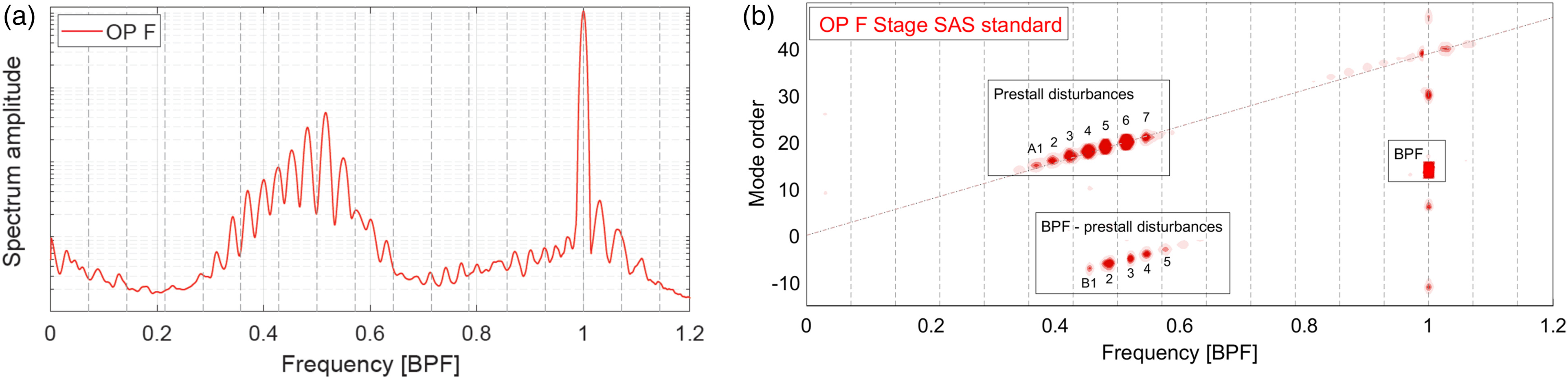
Focusing on the dynamic behavior, Figure 4a displays the pressure Welch spectrum of numerical probes at the casing for OP F (see Figure 2) in the LG setup. The prestall disturbances are also well reproduced by the numerical model. This can be seen when comparing Figure 4a with the highlighted OP 13 in Figure 3b. The equidistant spectral peaks match the frequency range of the experiments with a similar relative amplitude to the BPF. Additionally, the circumferential mode order for the same OP F is displayed in Figure 4b. Both the prestall disturbance branch (A1-A7) as well as its interaction with the BPF are marked. For instance, the dominant mode order is 20 for peak A6, meaning that a circumferential wave in its 20th harmonic has the highest amplitude for this OP. The frequency range and mode orders are also in good agreement with results previously obtained for the test rig (see Eck, 2020).

Figure 4.

Validation of numerical results for the large gap configuration. Stage CFD with large gap employing the SAS standard grid, OP F (see Figure 2). Frequency normalized by the blade passing (BPF). Engine orders are depicted by dashed vertical lines. (a) Pressure spectrum from casing probes and (b) Circumferential mode order.

Transient throttling

Compressors are subject to transient variation in mass flow during their operation, e.g. in acceleration and deceleration maneuvers. This change may bring a specific compressor stage for example from a choked state (high flow coefficient) to a stall-prone state (low flow coefficient). The rate with which this process occurs determines whether or not the system performance can be locally considered unsteady or quasi-stationary, for high and low throttling degrees respectively.

Figure 5 (left) shows the transient throttling path considered for the experimental campaign. Both NG and LG runs were performed. The process was repeated several times to make sure that the results are reproducible. The throttling rate implies a change of 0.1 in the flow coefficient Φ within circa 700 revolutions in the linear part.

Figure 5.

Experimental results for transient throttling of the stage. NG: nominal gap; LG: large gap. Left: performance parameters in time. Right: selected pressure Welch spectra for time windows labeled “a”, “b” and “c” (50 revolutions per bin), as shown in the left figure for the LG configuration.

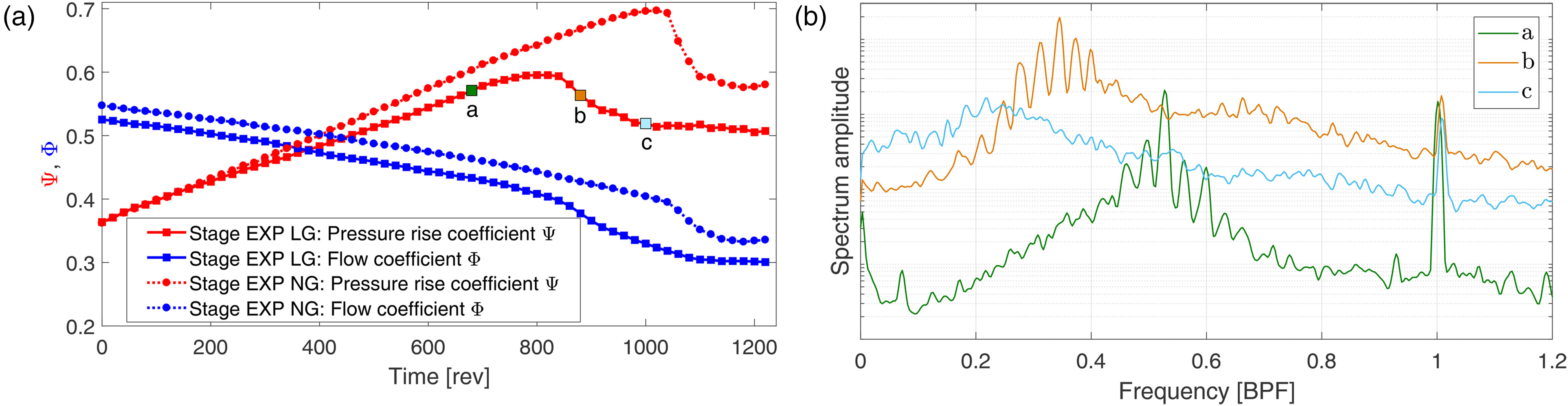
A few dynamic characteristics related to the clearance can be excerpted from Figure 5. First, the slope of the pressure-rise curve for the LG is slightly lower than for the NG case. Secondly, when comparing the curves starting from the same pressure-rise value, the NG configuration achieves on a later time a higher absolute Ψ level before the onset of stall. Furthermore, the drop in pressure rise after the beginning of stall is larger for the NG, while the LG experiences a comparatively milder reduction. Finally, the rate with which the flow coefficient Φ varies with the downstream transient throttling (slope of the blue curves) is similar for both clearance configurations. However, due to the larger flow blockage, the LG setup yields overall a slightly lower Φ value than the NG case.

To illustrate the frequency behavior, the Welch spectrum with a 50-revolution window was computed for three specific points labeled “a,” “b” and “c” on the left of Figure 5 for the LG setup. The corresponding spectrum is shown on the right part of the figure. At “a,” the typical prestall disturbance collection of peaks at approximately half the BPF is observed. Moving towards “b,” already after the maximum Ψ value, these peaks have moved towards a lower frequency range and the pressure amplitude has increase overall by one order of magnitude. At this point, part-span stall has already started. Finally at “c,” the rotating disturbance peak chain is much less pronounced and the pressure amplitude decreases in comparison to window “b,” however still higher than before stall. For this clearance configuration and throttling rate, no full-span or multiple large rotating stall cells develop.

Notice the similarity between the time-dependent throttling spectra for windows “‘a,” “b” and “c” on the right of Figure 5 and the constant throttling approach shown in Figure 3b. This indicates that the transient throttling rate employed experimentally was indeed able to reproduce a similar unsteady behavior to the runs with downstream boundary conditions fixed in time.

Computational methods

As described above, the compressor stage was validated in a former study employing a hybrid scale-resolving turbulence model with the full-annulus “standard grid.” For more details about these results, see de Almeida et al. (2024). This previous grid helped not only validating the performance and prestall spectral behavior of the test rig, but also pinpointing the flow regimes in which disturbances develop. Therefore, they paved the way for this work.

The main focus of the present simulations is on the much finer, “scale-resolving grid” suitable for Large Eddy Simulations (LES). Full-annulus meshing was also undertaken here, to comprise all feasible circumferential wavelengths and prevent phase errors linked to modeling just a few passages. Since the computational cost of LES runs is substantially higher than the previous URANS or hybrid setups, a compromise was made in that only the rotor row is modeled. Past investigations have shown that the stator presence is neither necessary for nor dominant in the development of prestall disturbances. The two critical flow coefficients at which these outset and separation occur will be different in the rotor-only case. This was accordingly taken into account when defining the appropriate boundary conditions in the current analyses.

The simulations consisted of 3D viscous, compressible runs using air as an ideal gas and the solver ANSYS CFX 2022R2. All computations were conducted with double-precision arithmetic. To prevent potential numerical reflections, the inlet is positioned approximately six rotor chords upstream of the spinner, while the outlet is situated roughly ten rotor chords downstream of the blade trailing edge. A longer extension was unnecessary according to preliminary studies. The inlet boundary condition consisted of a fixed total temperature and pressure, along with normal flow. Constant mass flow is enforced at the outlet, allowing for pressure variation, as expected in a near-stall setup with circumferential waves near the casing.

The modeling of turbulence is a key aspect in fluid dynamic regimes with high shear stresses and potential separation zones. This is the case with near- and in-stall flows assessed in this work. More specifically, the near-casing flow is not only affected by the endwall boundary layer, but also by the tip clearance jet, originated from the pressure gradient between the pressure and suction sides of the rotor blades. Adequate turbulence modeling in this particular region is key to comprehend prestall disturbances and its development into stall. Therefore, the grid was extra refined close to the rotor blade tip.

After preliminary tests, the LES approach considered here is the dynamic model as originally proposed by Germano et al. (1991) and Lilly (1992). In contrast to the classic Smagorinsky method (Smagorinsky, 1963), now the model coefficient Cd is no longer constant but rather computed locally in space and time, independently of user input. This grants the LES Dynamic model flexibility when dealing with complex flows with different turbulence regimes present concomitantly. In the current formulation, Cd is always non-negative and bounded by 0.04 to avoid overshooting.

The LES runs are initialized from previous unsteady SST simulations, already periodically converged, with 5% turbulence intensity implemented at the inlet. No further turbulent production methods (such as artificial vortices) were applied in inflow regions for the LES runs, following other work (Montorfano et al., 2013; Gan et al., 2016). This choice was made since the turbulence-developed initial conditions and the specific flow regime linked with prestall disturbances were already enough to sustain the production of turbulent structures, especially at the blade tip. The boundary conditions were also kept the same as in the former study for validation consistency. Additionally, one requirement for the present simulations was that the prestall disturbances develop inherently within the stage, independently from explicit and potentially misleading time-dependent variations in boundary conditions. Preliminary runs have shown that some unsteady patterns in the inflow plane could strongly influence and even “artificially” trigger the onset of prestall disturbances and even stall. The good agreement with experiments showed that this strategy was effective.

The LES approach considered here is wall-modeled, so that the focus is not in the boundary layers themselves, but on the relatively larger turbulent flow structures developing close to the casing. This choice helps reducing the computational cost substantially. More comments on the boundary layer modeling will be provided later. Unfortunately there is no available full-annulus simulation for this setup solving walls with LES grid precision, since the order of magnitude in processing power would be unfeasible, even with modern high-performance facilities such as the one employed in the present simulation campaign. Even though a direct comparison is not yet possible, attention was paid to specific scale-resolving grid requirements as discussed in the following section.

A bounded central difference scheme is employed when integrating the advection terms. The time march is the second order backward Euler, with up to six inner iterations at each time step. Considering CFL restrictions and preliminary tests, the rotor passing period is modeled with 100 time steps, providing enough time resolution but also taking into account the large computational resources required for the long transient runs.

Grid description

The unstructured mesh was generated with Numeca’s AutoGrid5. Conformal blocks were produced, to avoid flux splitting errors. Circa 380 layers were defined from hub to shroud, while 176 nodes cover the axial dimension of each blade. Approximately 1,300 cells are located in the circumferential direction for each radial layer. To improve the spatial resolution close to the tip clearance, 130 radial elements were defined in the rotor gap. In total, the full-annulus scale-resolving grid has 140 million cells.

Conventional URANS simulations are usually preceded by a straightforward grid independence study, in which several meshes with different spatial resolutions are generated, some representative scalar for the whole problem is computed and compared. Sometimes an additional parameter to indicate a confluence of results with refinement is also presented, such as the Grid Convergence Index (see Celik, 2008).

Scale-resolving grids, however, must satisfy a few other model-specific prerequisites. The first aspect is the number of cells conveying the integral length scale. The latter is defined as

To illustrate the integral length scale distribution for the rotor, Figure 6 depicts on the left its values for a representative LES run with the LG configuration. Only cells with 2Δ≥l0 are shown, colored by their radial position, to ease the visualization. According to the reasoning above, these elements would not adequately represent the eddies in a scale-resolving turbulence model. They are however clearly restricted to the boundary layers, which are not the principal target of the present wall-modeled LES simulations. Indeed, the main goal is to achieve good eddy resolution close to the tip clearance, capturing the comparatively larger scale dynamics of prestall disturbances and stall. The mesh in this region is adequately covered with several cells solving the integral length scale. The right half of Figure 6 show mesh surfaces edges for the rotor blades, hub and part of the shroud.

Figure 6.

Left: cell volumes solving two times or less the integral length scale. They accumulate close to the walls and are colored by their radial position to ease visualization. Right: selected surfaces from scale-resolving grid.

A second metric ensuring proper scale-resolving turbulence modeling is the ratio between TKE solved by the grid and total TKE. For the present mesh, a threshold of 80% was targeted, so that almost the entire domain models 20% of less of the TKE not solved by the discretization itself. Particular attention was given to regions close to the rotor shroud.

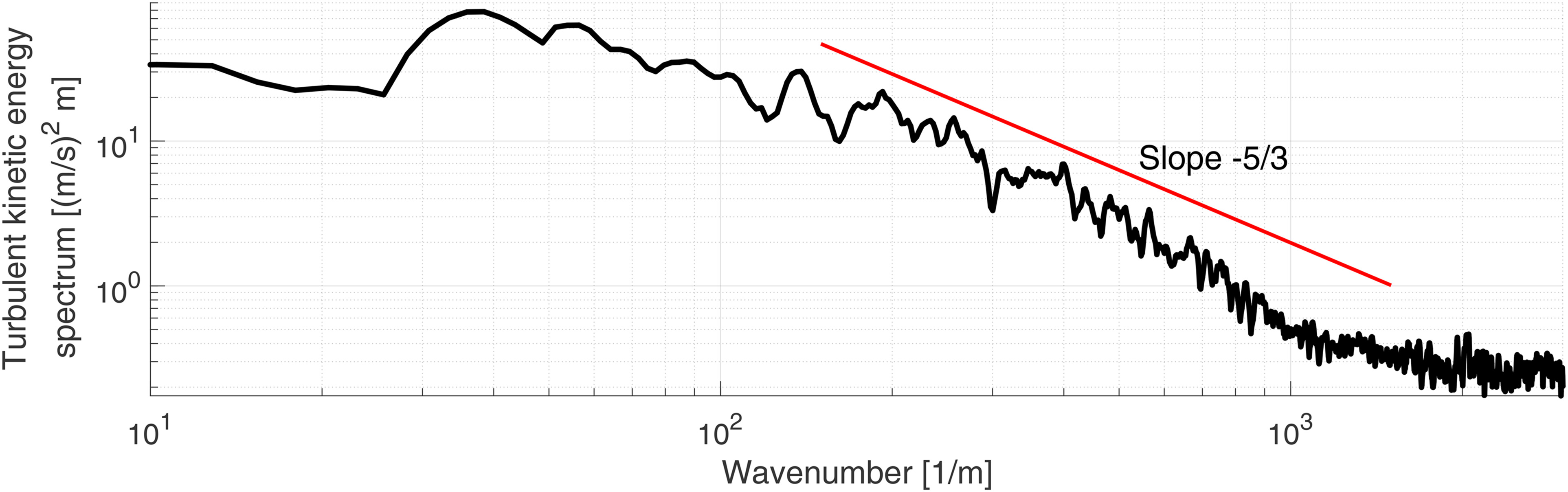
The third mesh criterion is related to the TKE spectrum for the runs. Considering the same LES case from Figure 6, the spectrum for the TKE was computed for multiple probes positioned at various circumferential locations at the rotor clearance. This is shown in Figure 7, taking Taylor’s frozen turbulence hypothesis into account (see Taylor, 1938). The theoretical “−5/3” prediction from Kolmogorov is also added to the figure, showing a good spectral agreement with the numerical results, particularly for the inertial subrange.

Figure 7.

Turbulent kinetic energy spectrum for sensors in the rotor tip clearance for a LES run. The mean of several probes is computed and the red line represents Kolmogorov’s theoretical prediction for the inertial subrange.

Finally, the CFL condition must also be considered to guarantee good time resolution. For the present case and particularly near the rotor clearance, CFL values close to one were obtained. Tests with smaller time steps did not change the flow dynamics substantially, so that the time resolution mentioned above was kept as a good compromise between accuracy and computational costs. Meeting all the above criteria clears the way for reliable LES simulations.

Transient throttling

One fundamental difference between experimental campaigns and simulations should be highlighted. On the one hand, as typical from turbomachinery measurements, results for a longer time span can be gathered (usually with a limited number of physical probes). Unsteady numerical investigations, on the other hand, are normally restricted to a much smaller time window (with the benefit of having almost all flow quantities in the entire domain readily available).

This limitation on computation resources is particularly relevant for the present full-annulus scale-resolving simulations. Therefore, the change in mass flow implemented in the CFD runs is much quicker than the throttling rate achieved in the test rig. More specifically, the numerical boundary conditions provide a variation of 0.1 in the flow coefficient Φ within approximately 15 rotor revolutions. Even this relatively short time period, due to the fine mesh employed, took several months in a high-performance cluster with circa thousand CPU cores running in parallel. Figure 8 depicts the pressure rise and flow coefficient time trace for the simulations, for both NG and LG setups. The mass flow at the outlet was reduced linearly considering values yielding a flow field in which prestall disturbances develop, moving then into part-span stall. Despite the larger throttling rate in comparison with the experiments, some flow characteristics linked to prestall disturbances and stall onset can still be identified. Additionally, the results can also be contrasted with scale-resolving simulations considering fixed boundary conditions (see de Almeida and Peitsch, 2024).

Figure 8.

Performance results for transient throttling simulations with the rotor LES scale-resolving full-annulus setup. NG: nominal gap; LG: large gap.

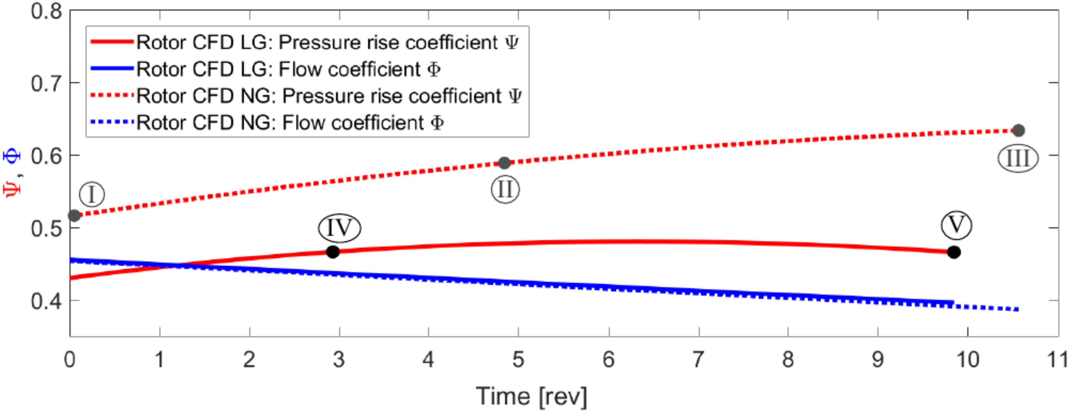
The fact that the flow coefficient lines for the NG and the LG setup now partially overlap is a mere coincidence related to the throttling value (mass flow) chosen at the time origin. In other words, a horizontal shift in Φ would take place if the initial throttling level was different. The results presented later are in any case independent of the choice of the starting time.

In comparison with Figure 5 for the experimental campaign, the pressure rise values shown in Figure 8 for the numerical setup are overall lower. This is expected since the computational domain does not include the stator vanes, which further increase the fluid static pressure. It is also possible to see that, for the boundary conditions implemented, Ψ reaches a maximum and already starts to fall for the LG setup. The pressure rise for the NG counterpart is also at the verge of starting to decline, since flow separation begins to develop in the last revolutions.

To confirm this, three snapshots were selected from the transient throttling run for the NG configuration, as shown in Figure 9. They correspond to OP to as shown in Figure 8, respectively from prestall-disturbed to part-span stall regimes. It is possible to see in the vorticity surface distribution (left part of Figure 9) that the tip clearance jet plays a dominant role in the production of small eddies at large radii. While at OP the jet is still contained within each passage, the eddy influence area (both in its axial and radial extents) increases with lower flow coefficient, up to the point in OP where the small vortical structures start to spill forward along the leading edge (LE) of the adjacent blade. In other words, the blockage rise at high radii is responsible for increasing the main flow incidence, forcing a deviation of fluid particles away from the axial direction. This process establishes for all blades, which are indeed dynamically “connected” by the tip clearance and the flow upstream the LE plane.

Figure 9.

Operating points for nominal gap (NG) rotor LES scale-resolving setup with full-annulus grid. Labels according to Figure 8. Left: 3D surfaces for instantaneous vorticity colored by the circumferential velocity (low values for rotation opposing the rotor). Right: limit streamlines on rotor blades.

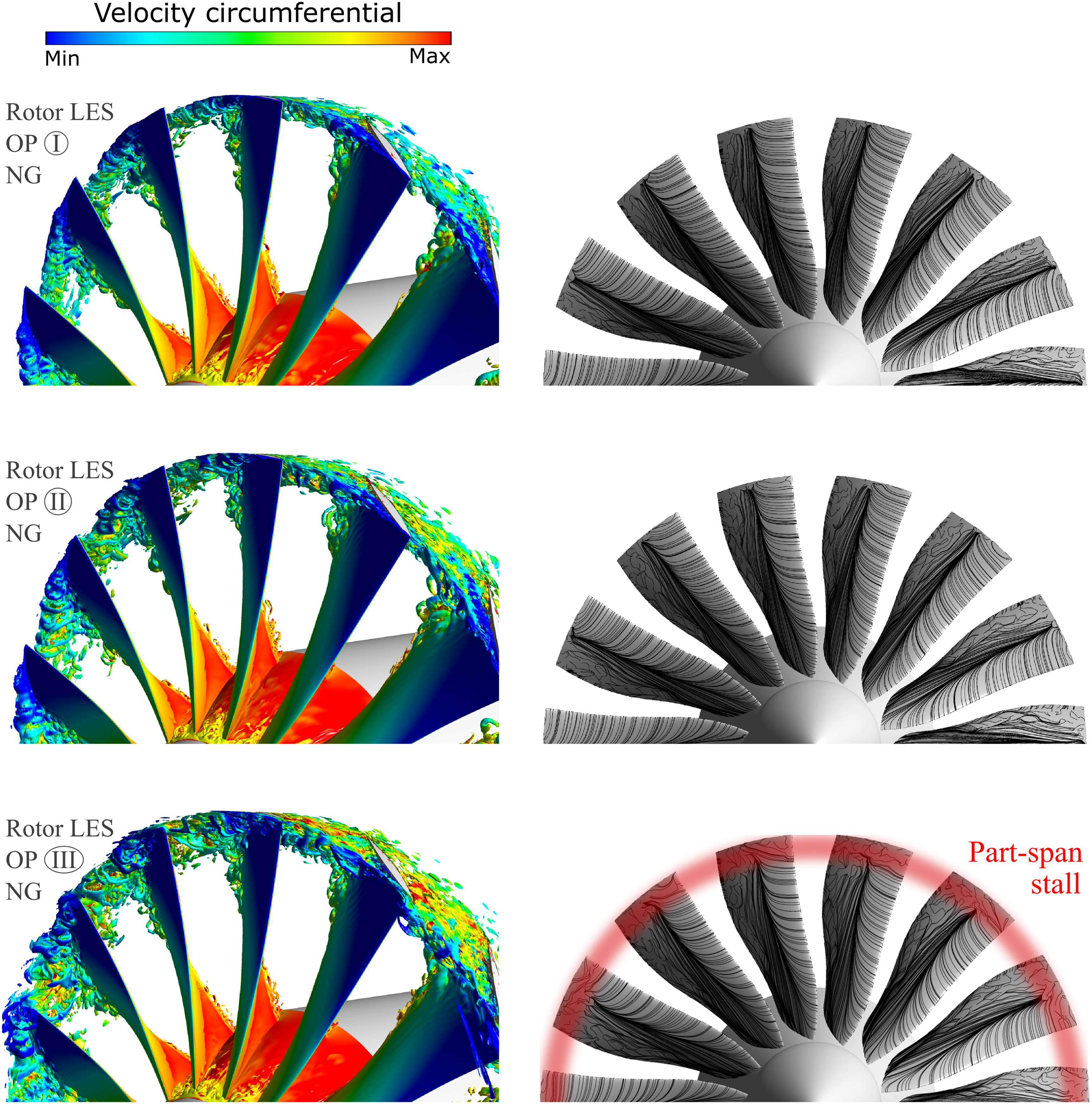
The right part of Figure 9 shows the limit streamlines on the blade rotor. For all OPs shown, an intense radial migration occurs from small to large radii. A separation line is also visible around half chord. This is characteristic from this particular design and has been already mentioned in the previous study (see de Almeida et al., 2024). The eddy production linked to this mid-chord separation, especially for the upper half of the blade, is also clear from the vorticity surface distribution. At OP and OP , the flow is still attached at the LE. However, at OP LE separation takes place close to the blade tip (indicated by the shaded red annulus). The flow along the lower span is still attached at the LE. A similar scenario is observed for the LG setup, not shown here for brevity.

When transient throttling the compressor stage, the question arises of when prestall disturbances and then stall establish. According to a previous study from de Almeida et al. (2024), an hypothesis was proposed, claiming that when blockage volumes (here represented by time-averaged axial velocity equals null) in the clearance of each blade merge into a single surface spanning the whole circumferential extent, then prestall disturbances can be detected in the pressure spectra.

To conceive this situation, three OPs for the LG setup are shown in Figure 10. The 3D surfaces correspond to locations where the time-average of the axial velocity is zero. They are colored here by the time-averaged radial velocity to ease the visualization of the tip clearance jet. The negative regions (marked in blue) convey vectors pointed inwards, while the positive regions (marker in red) point outwards to higher radii. A parallel stream of negative and positive values at the clearance pinpoint the tip jet (in a time-average sense), as shown in the upper-right corner of Figure 10.

Figure 10.

3D surfaces in which the temporal average of the axial velocity is zero, colored by the radial velocity component. Positive values point outward. OP labels according to Figure 8.

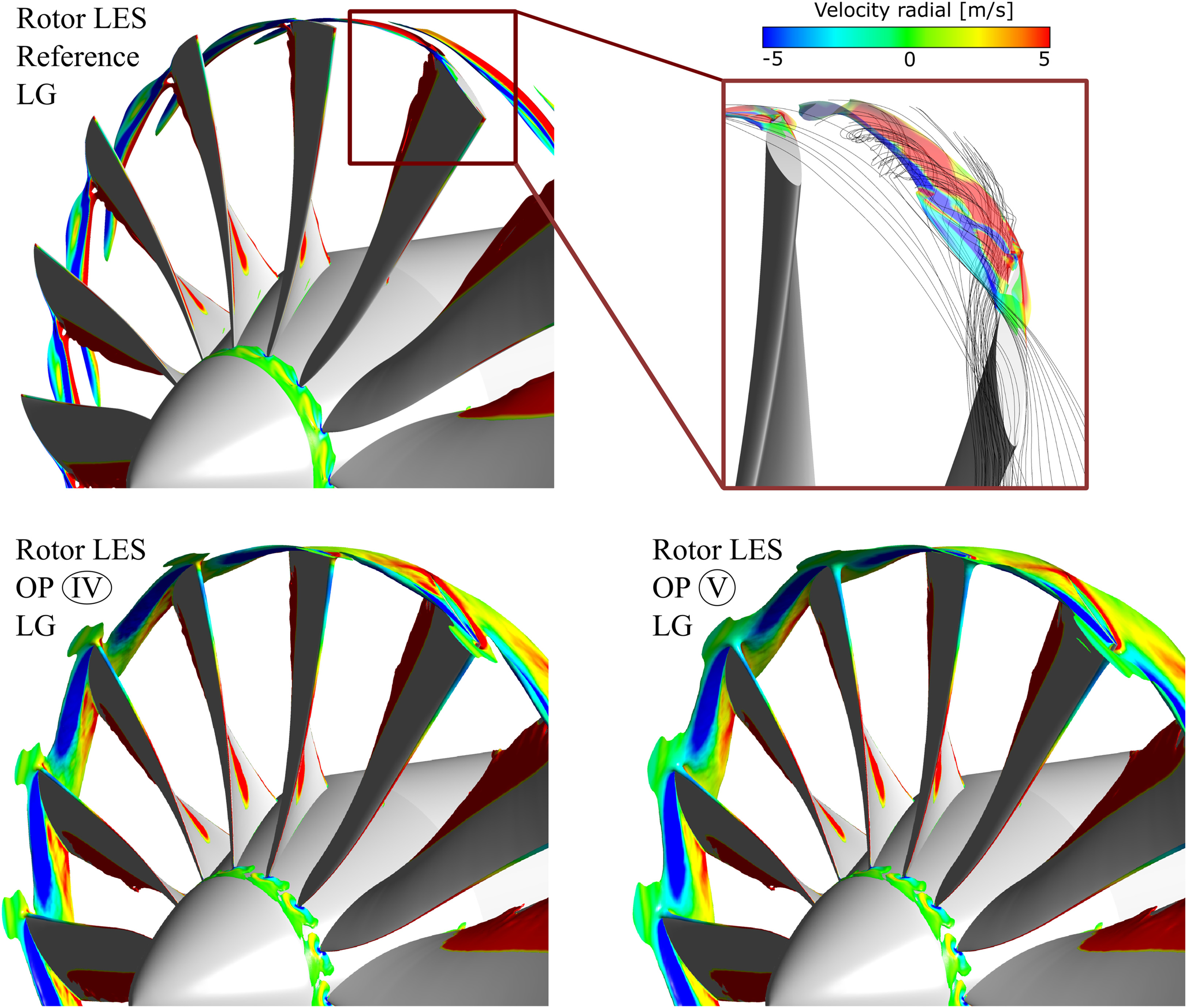
The first OP at the upper left is not part of the transient throttling results, but rather a reference state with constant boundary conditions for relatively high flow coefficient. It indicates a regime in which the rotor tip is not yet intensively loaded. It is clear that each of the tip clearance jets are still contained in the respective blade passage, and the 3D surfaces are not connect to the adjacent counterparts.

OP (as indicated in Figure 8) represents a state with a flow coefficient smaller than the reference case. Now the 3D blockage surfaces are not disconnected but merged into a single one covering the entire clearance region for all blades. This condition is linked to the presence of prestall disturbances in the signal (as discussed by de Almeida and Peitsch, 2024; de Almeida et al., 2024 for constant throttling cases). It is nevertheless clear that the tip clearance jet is still mainly contained within each blade passage.

With further throttling, OP shows the leading edge spillage in a time-average sense. The blue region indicating the upstream boundary of the tip clearance jet becomes parallel to the LE plane. That is, due to the higher blockage, the incidence of the fluid particles is increased, forcing them to stream towards the adjacent blade passage (in the counter clockwise direction, as seen from the front). This additional loading is enough to induce flow separation at the LE, close to the tip (image not shown here for brevity, but similar to the part-span stall depiction in Figure 9). Further throttling then increases the span of the separated region.

The spectrum for the transient throttling, due to the short query window, is not as sharp as the spectra for long runs with constant throttling boundary conditions. However, a similar behavior is seen, in which disturbances with relatively smaller amplitudes develop (as in OP ) before the onset of part-span stall and higher flow fluctuations (as in OP ).