
Introduction
Aviation faces possibly the most difficult decarbonisation challenge of all sectors for 2050 due to the increasing traffic growth coupled with a lack of carbon-free alternative solutions. Inaction on aviation will place a further strain on a country’s ability to achieve EU climate targets, such as the ‘Fit for 55’ targets for 2030 (European Economic and Social Committee, 2021), and the European-wide target of net-zero flights by 2050 outlined in the Destination 2050 report (A4E, 2021). These climate targets are set in the context of a growing aviation industry, with aircraft traffic predicted to increase up to 3.1% annually, reaching 10 billion passengers by 2050 (ATAG, 2021), making the challenge increasingly more complex and the solution more urgent. Islands such as Ireland are in a unique position where there is no alternative to air travel in the context of Flight-Path 2050 interconnectivity goals, which aim for a 4-hour trip door-to-door anywhere in Europe (European Commission, 2011). The importance of aviation to Ireland’s economy cannot be understated; Europe’s largest airline contributes to over 26,000 jobs annually, carrying 20 million passengers to and from the island where guests spend €1.5 billion per year (Ryanair, 2023b). Furthermore, over 50% of the global market share for aircraft leasing is located within Ireland. Given this context, it is important that Ireland becomes a leading-voice in the sphere of sustainable aviation.
Sustainable Aviation Fuel (SAF) is envisaged to be the main driver of decarbonisation towards 2050, and is projected to offset 53–71% of aviation’s carbon emissions (ATAG, 2021). SAF can be further categorised through its method of production; bio-SAF, manufactured through hydrogenation of bio-derived feedstocks, or Power-to-Liquid (P2L) SAF, manufactured via synthesis of green hydrogen with carbon, ideally sequestered from the atmosphere in a process known as Direct Air Capture (DAC), which can be powered entirely from renewable electricity. Green Liquid Hydrogen (LH2) is another sustainable P2L solution for aviation, which is included alongside SAF in the ReFuelEU mandates for 2030 and 2050 (European Parliament, 2023). These mandates target 6% sustainable fuel uptake at airports by 2030, which increases to 70% by 2050 – furthermore, sub-mandates for P2L fuels are set at 1.2% for 2030, rising to 35% in 2050 (European Parliament, 2023). Although bio-SAFs are likely the best near-term solution, which is reflected in the ReFuelEU mandates, P2L fuels are the primary focus of this study. This is due to their low Carbon Intensity (CI) when produced using renewable electricity, and due to uncertainty surrounding the long-term sustainability of SAF produced with bio-derived carbon feedstocks (ICCT, 2019; Imperial College London Consultants, 2021). Furthermore, the untapped potential of off-shore wind generation within Ireland, at a theoretical annual output of 2,852 TWh, provides a valuable opportunity to become a leader in P2L fuel production (National Hydrogen Strategy, 2023).
Although both P2L solutions offer a tangible decarbonisation solution, there is uncertainty over their economic viability due to the challenges associated with each technology – P2L SAF requires significant energy input for its production (Grim et al., 2022). On the other hand, LH2-powered aircraft introduce challenges in the provision of infrastructure and aircraft design as LH2 is not a drop-in alternative to kerosene, while also suffering from in-flight performance penalties due to the reduced energy density of the fuel, and the storage of a cryogenic fuel within the fuselage (Mukhopadhya and Rutherford, 2022). Previous studies compared the market coverage and design mission performance of LH2 aircraft against kerosene and SAF (Karpuk and Elham, 2022; Mukhopadhya and Rutherford, 2022), however the published literature lacks a comprehensive analysis of the real-world energy performance of these technologies.
Therefore, this study aims to quantify the real-world performance of LH2 and SAF technologies by means of an operational case study for a short-haul European airline. The operational case study consists of a fleet-wide evaluation of a full day of airline operations, considering all flights to and from the island of Ireland for LH2 and SAF scenarios, where the fleet-wide performance is measured in terms of fuel energy consumption and total energy consumption, also known as the Well-to-Wake (WtW) energy consumption. Specific objectives of this study include:
Development and validation of CFM56-7B26 and LEAP-1B27 propulsion system models
Development and validation of Boeing 737-800NG and Boeing 737-8200 MAX aircraft models
Calibration of the baseline aircraft models with respect to real-world flight data
Development of LH2 propulsion system and aircraft models with varying LH2 tank Gravimetric Index (GI) values
Development of an Intercooled-Recuperated Engine (IRE) variant of the LH2 propulsion system
Fleet-wide energy analysis across the complete operating schedule for SAF and LH2 aircraft configurations
Analyse the impact of fuel choice, aircraft technology level, GI values, and IRE-propulsion on the outcomes of the study in terms of energy and cost.
Methodology
Aircraft model
Aerodynamics
A representative model of the B737-800NG (B737-NG) and B737-8200 MAX (B737-MAX) aircraft were developed using the open-source Stanford University Aerospace Vehicle Environment (SUAVE) conceptual design tool (Lukaczyk et al., 2015), where details of the aircraft geometry were obtained from airport planning reference sheets (Boeing, 2023). SUAVE contains suite of physics-based and semi-empirical methods for aerodynamics, propulsion, and mission analysis calculations (Lukaczyk et al., 2015). The physics-based ‘fidelity-zero’ Vortex-Lattice Method (VLM) within SUAVE, which has been previously validated against wind tunnel experimental data (Botero et al., 2021), was used to model the inviscid lift and induced drag of the aircraft wings and stabilisers. This VLM model is based on a modified version of the NASA VORLAX code (Miranda et al., 1977). Semi-empirical methods within SUAVE were used for the aircraft drag build-up based on correlations provided by Shevell (1983), Lukaczyk et al. (2015). Correction factors within these semi-empirical drag calculation methods were utilised for calibration of the aerodynamic model, as discussed in a later section. An example of a semi-empirical method used to calculate the fuselage parasite drag is outlined in Equations 1 and 2 where
Propulsion
An enhanced-fidelity propulsion system model of the CFM56-7B26 and LEAP-1B27 turbofans were developed using NASA’s Numerical Propulsion System Simulation (NPSS) tool (Jones, 2007). The generic turbofan model, illustrated in Figure 1a, was designed within NPSS, and incorporated generalised component performance maps developed in NASA’s energy efficient engine programme to characterise the off-design performance (Batterton, 1984). The model was calibrated by tuning the design variables of each engine component labelled in Figure 1a, such as the pressure ratio, isentropic efficiency, combustor temperature, and bypass ratio, along with desired blade/vane temperatures which were used to calculate the compressor bleed flows for turbine cooling requirements using NASA’s CoolIt algorithm within NPSS (Gauntner, 1980). The calibration aimed to minimise the error between the model’s Thrust Specific Fuel Consumption (TSFC) predictions and the experimental TSFC results for Sea-Level Static (SLS) operating points obtained by the International Civil Aviation Organisation (ICAO) (EASA, 2023), while ensuring the target thrust requirements were achieved for each design point. The TSFC validation results for the CFM56 and LEAP SLS operating points, alongside Top-Of-Climb (TOC) and Rolling Take-Off (RTO) are presented in Table 1. The prediction accuracies of the high-powered SLS-100% and SLS-85% operating points ranged from 0.28%–0.67%, whereas the SLS-30% and SLS-7% operating points, which are less critical due to the lower fuel-flow values, and lower representation of these operations throughout the flight envelope, were predicted with accuracies ranging from 0.44%–4.25%.
Figure 1.
(a) Generalised propulsion system model for CFM56-7B26 and LEAP-1B27 turbofan models (b) Intercooled-Recuperated engine configuration for hydrogen-powered aircraft.
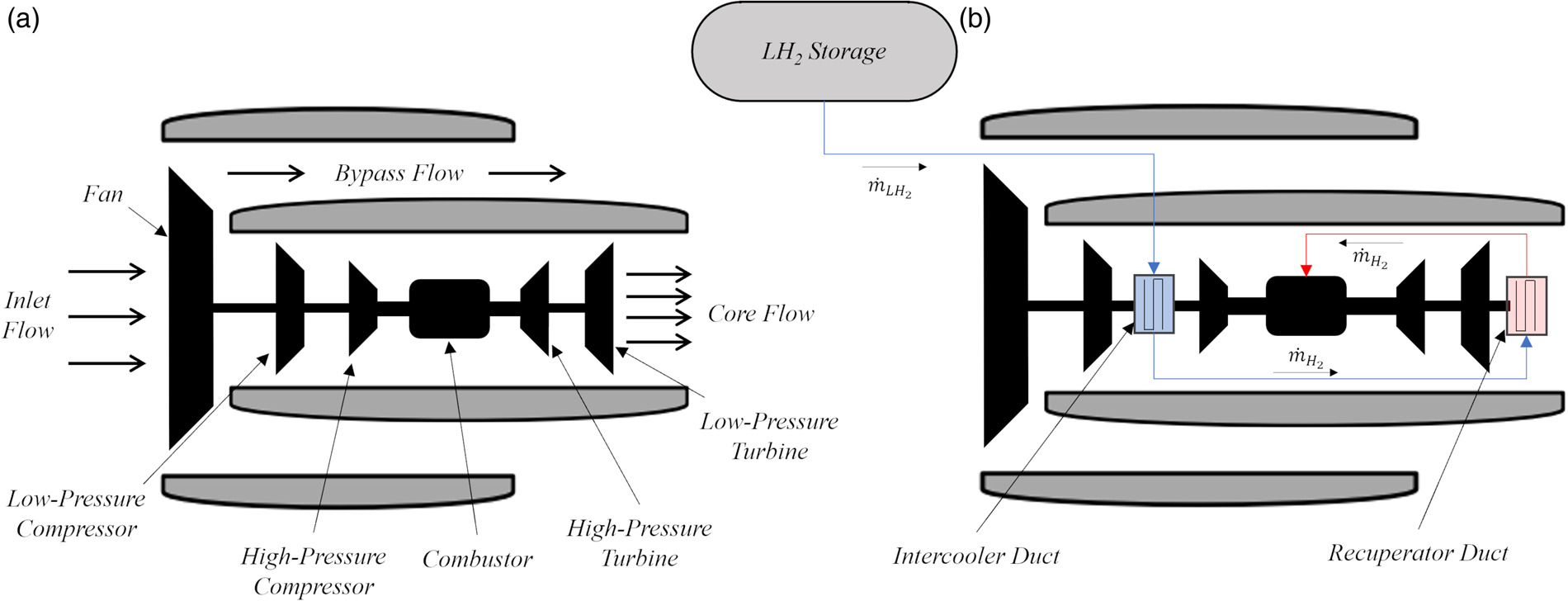
Table 1.
Validation results for NPSS turbofan models against ICAO data.
Following the development of the standard propulsion system models, equivalent LH2 models were developed for the CFM56 and LEAP engines by increasing the Lower Heating Value (LHV) of the fuel from 42.8 MJ/kg for Jet-A to 119.96 MJ/kg for hydrogen (Cecere et al., 2014). Hence, only the specific energy was accounted for in the development of the baseline LH2 propulsion model, with no further modifications to the engine (i.e., the fuel was considered as an energy carrier only). An LH2 Intercooled-Recuperated Engine (IRE) configuration was also developed through the addition of compact Heat Exchanger (HEX) ducts in between the Low/High-Pressure Compressors (LPC/HPC), and behind the Low-Pressure Turbine (LPT), as illustrated in Figure 1b. The IRE model setup is discussed in greater detail in a later section. The baseline kerosene models were simulated at a full range of operating points, including delta temperatures compared to the International Standard Atmosphere (ISA), i.e., ΔTISA values of ±10°F and ±27°F to facilitate the fuel-flow validation of the total aircraft model against real-world operations, which is discussed in a later section. The LH2 propulsion systems were simulated only at ISA temperatures.
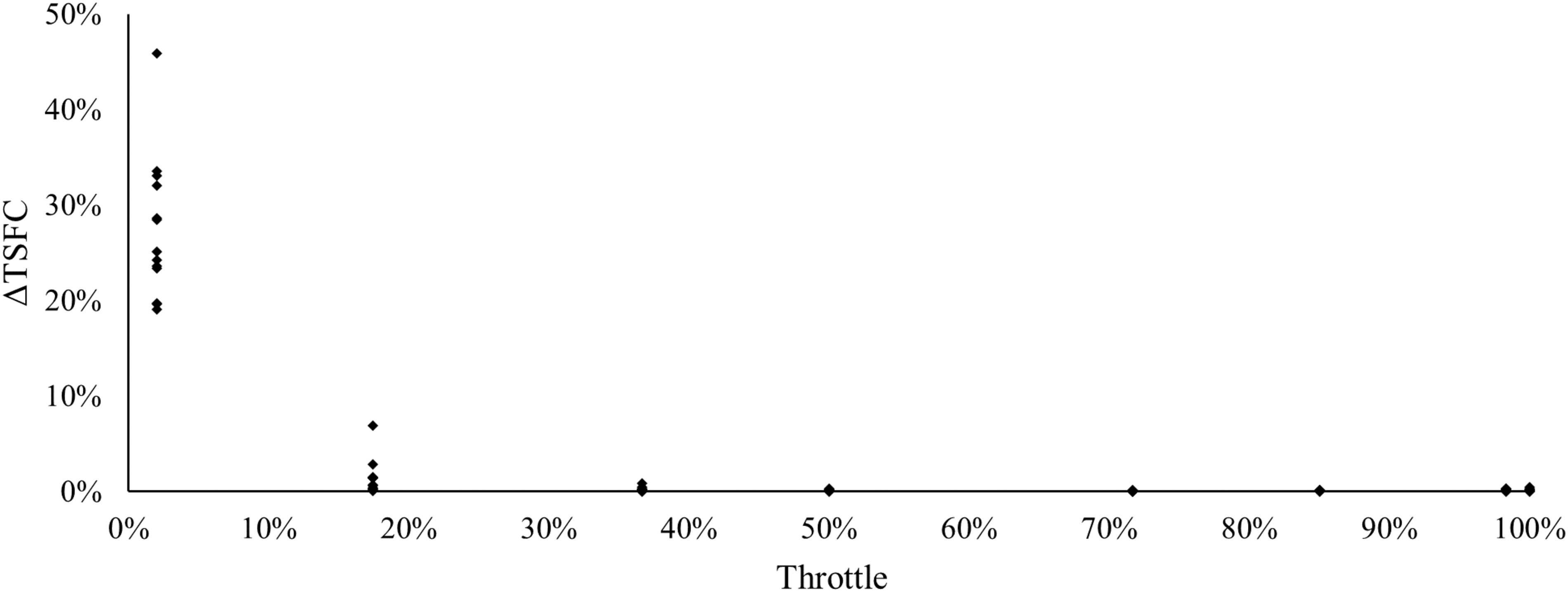
Surrogate models representing the thrust and TSFC of each engine configuration were generated in order to connect the NPSS models to SUAVE, and were generated using Gaussian regression methods (Rasmussen and Williams, 2006). Initially the ΔTISA values were included within the surrogate model formulation, however this resulted in prohibitively slow surrogate model evaluations for the current study. Instead, to include the temperature effects, separate surrogate models were developed for ΔTISA values of 0, ±10°F and ±27°F, where the final thrust and TSFC predictions within the real-world operations model were generated through linear interpolation between the outputs of the appropriate models. This method generated improved accuracy compared to not including temperature effects, while maintaining sufficient computational efficiency. The final surrogate models yielded r-squared values >0.9999, and the models were tested against a range of unseen test data. The test data consisted of 104 operating points at a range of unseen altitude, Mach numbers, throttle, and temperature values, in order to evaluate the maximum possible surrogate prediction errors. Figure 2 shows the relative prediction errors for the kerosene-powered LEAP surrogate model against the NPSS model simulation outputs, where 85/104 points were predicted with <1% error, with the majority of these almost equal to 0%. All 19 points with >1% error were for operations below 20% throttle, with 13 of these points at 2% throttle. Although there are significant errors for the 2% throttle operations, the fuel-flow rates for these operations are low and have a negligible impact on the overall fuel burn prediction accuracy over a complete flight, which is observed during the validation of the total aircraft model. Therefore, the surrogate modelling method was deemed to be an acceptable trade-off for prediction accuracy against computational efficiency.
Real-world operations
The real-world operations model in this study represents a key novel aspect of this research. This work aims to enhance the coupling between aircraft conceptual design and flight operations, to predict the real-world benefits obtained with each technology, and identify the key technology drivers of decarbonisation for a given operational strategy. The real-world operations model was developed to generate flight paths for the SUAVE mission analysis module, based on the actual flight paths and Take-Off Weight (TOW) of the airline’s flights. This study uses a similar approach to the author’s previous work (Gallagher et al., 2023b), albeit with a significantly larger flight database, and improved flight data derived from on-board Quick-Access Recorder (QAR) data, compared to the publicly available Automatic Dependent Surveillance-Broadcast (ADS-B) data used in the previous study – which did not account for the true airspeed of each flight.
Flight database
An extensive flight database was provided to the authors by Ryanair, consisting of QAR data for a full day of B737-NG operations (2,457 flights), alongside a further 23 B737-MAX flights, with a data sample rate of 1 Hz and 11 Hz, respectively. Ryanair are Europe’s leading airline in terms of flights and passengers carried, operating almost 3,000 flights daily with a fleet of 548 Boeing 737 aircraft (EUROCONTROL, 2024; Flightradar24, 2024). The flight database provided a valuable opportunity to conduct a rigorous validation and calibration study to evaluate and maximise the accuracy of the selected conceptual design tool, alongside detailed operational case-studies. The distribution of mission range and TOW within the flight database is illustrated in Figure 3, where the TOW values are redacted due to the sensitive nature of the data, but the variation of TOW values is indicated on the graph. There was significant variation in the mission range, ranging from 88 NM to 2,320 NM, with an average mission range of 693 NM, which is closely aligned to the airline’s annual average mission range of 766 NM in 2023 (Ryanair, 2023a).
Figure 3.
Distribution of range and TOW of the B737-NG flight database and calibration/test datasets.
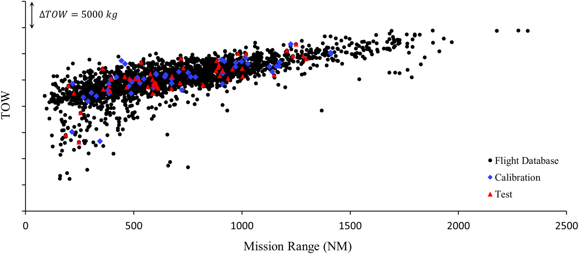
To perform the calibration of the B737-NG aircraft model, a subset of 50 B737-NG flights were selected from the flight database and place into the calibration dataset using a random sampling method. In order to maintain sufficient representation of the wider database, the calibration dataset was generated such that the mean of the mission range and TOW were kept within 1% of the complete flight database, while the sample standard deviations were maintained within 10% of the complete flight database, which was achieved through generation of thousands of random samples. The 50 selected flights are illustrated in Figure 3, superimposed on the complete flight database. Using the same approach, a further 50 flights were placed in the B737-NG test dataset. Due to the limited available data for the B737-MAX aircraft, 19 flights were manually selected and placed in the calibration dataset, leaving four remaining flights that were placed in the test dataset.
Flight path approximation
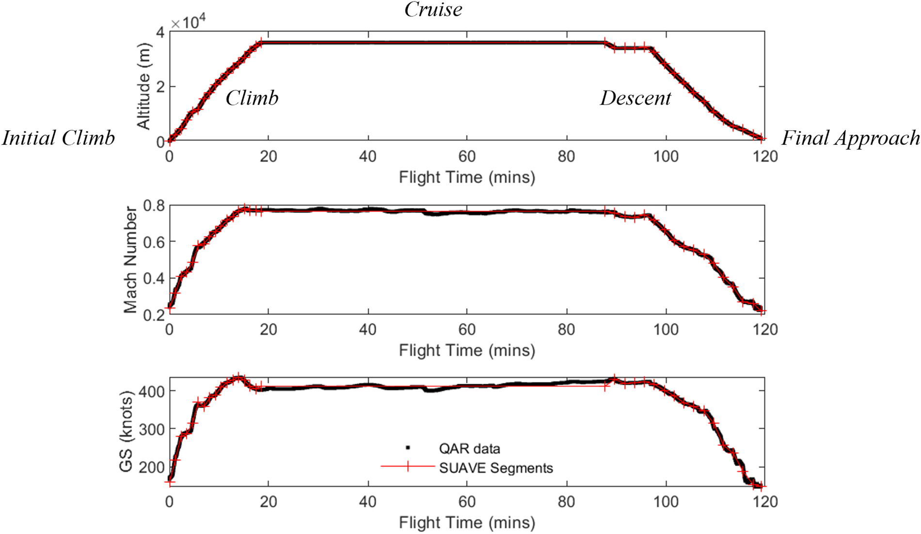
In order to simulate each of the real-world flights within SUAVE, the flight paths were approximated in terms of piece-wise linear sub-segments which were input into the SUAVE mission analysis module. The flight paths were approximated in terms of altitude, Mach number, and Ground Speed (GS) with respect to the flight time, where 15 sub-segments were used for the climb and descent phases, and a variable number of cruise and step-climb segments were used to accurately capture the cruise profile. The first and last sub-segments represented the initial climb and final approach segments, respectively, which were separated from the climb/descent segments to account for the deployment of the flaps, slats and landing gear. Note that the take-off and landing ground segments were not considered in the real-world operations model.
Figure 4 shows an example flight path approximation of a multi-cruise flight with step-climb segments. The linear SUAVE flight paths were approximated using a least-squares approach in an automated MATLAB software routine, formulated using the QAR flight data. The generated SUAVE segments are highlighted in Figure 4, which show good agreement with the actual flight paths obtained from the QAR data. The flight segments within the climb and descent phases were simulated using a linear-Mach number and constant rate of climb/descent, whereas the cruise segments were simulated using a constant Mach number and constant altitude. During the flight simulations, the linearised equations of motion were solved to achieve convergence for each segment within the mission. More details on the SUAVE mission simulation process can be obtained from Lukaczyk et al. (2015).
Model validation and calibration
Preliminary validation
A preliminary validation of the B737-NG and B737-MAX models was conducted to assess the fuel-flow accuracy of the uncalibrated model over a broad spectrum of range of real-world flight data. To the authors’ knowledge, no such validation exists in the published literature for a physics-based low-fidelity model, which represents a further novel aspect of this study. The preliminary validation model consisted of the standard, uncalibrated SUAVE aerodynamic model, combined with the NPSS propulsion surrogates and the real-world operations model for the mission analysis. A sample flight validation with normalised fuel-flow values is presented for the B737-NG and B737-MAX models in Figures 5a and 5b, respectively. The average fuel-flow error magnitude per segment and the average mission fuel burn error magnitude for each validation sample set is presented in Table 2. Note that the uncertainty of each fuel-flow measurement within the actual flight data was ±2 lb/hr.
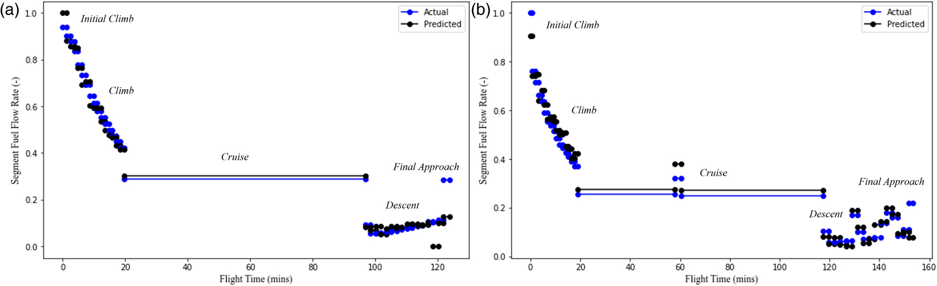
Table 2.
Preliminary validation of uncalibrated model fuel-flow predictions for calibration and test datasets for B737-NG and B737-MAX models against actual flight data.
The average mission fuel burn for the test dataset of each aircraft configuration is relatively low at 2.2% and 4.9% for the B737-NG and B737-MAX aircraft, respectively. However, from observing the segment fuel-flow errors, it is clear that more significant inaccuracies exist within the initial model. The majority of the fuel-flow error for the initial climb and final approach segments can be attributed to the flaps/slats and landing gear deployment, which was not accounted for in the preliminary model. Significant fuel-flow errors also occurred during the descent segment, partially due to inaccuracies representing the idle throttle fuel-flow, but more so due to several negative throttle segments output by the SUAVE mission solver, which are represented as zero fuel-flow as observed in the second-last descent segment in Figure 5a. Such negative throttle segments indicated that there was insufficient drag to perform the deceleration that occurred in the real-world flight path, hence, convergence was achieved through negative drag, represented by a negative throttle value. Despite these errors, it is clear from Figures 5a and 5b that the aircraft model showed consistent performance over the climb and cruise segments, and therefore model inaccuracies were possibly due to the drag build-up methods which were based on the semi-empirical correlations previously noted in the aerodynamics section.
Calibration
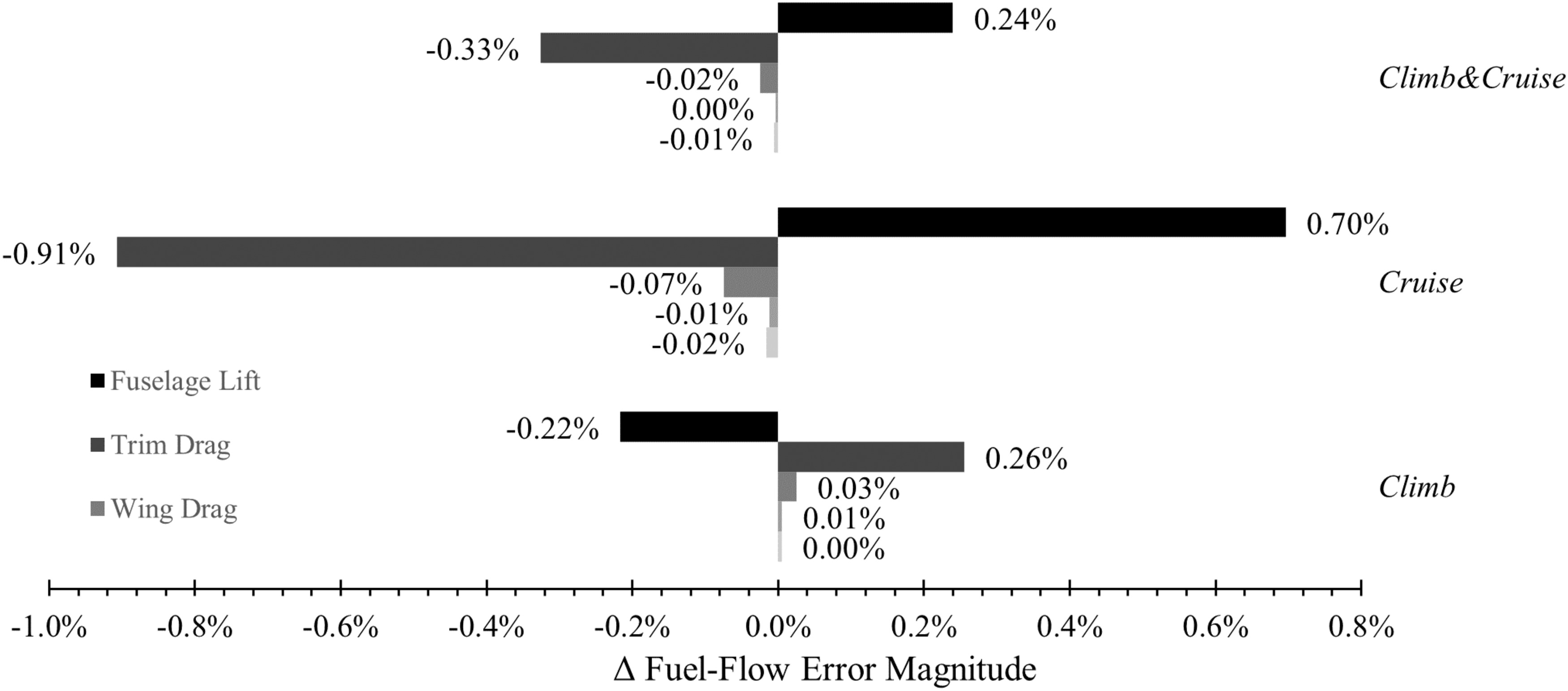
The aerodynamic coefficients associated with the semi-empirical methods used for the drag build-up were optimised in order to minimise the average predicted fuel-flow errors against the real-world flight data, following a similar method used in previous work (Gallagher et al., 2023b). The aerodynamic model calibration utilised the B737-NG data due to the limited available data for the B737-MAX aircraft, where the average climb and cruise fuel-flow relative error magnitudes were minimised using the Sequential Least-Squares Quadratic Programming (SLSQP) minimisation algorithm in the SciPy Python library, using a custom multi-start algorithm where initial values were populated using a Latin hypercube sampling method. Five empirical coefficients, related to the fuselage lift factor, trim drag, wing and fuselage form factors, and the viscous lift-dependent coefficient, were varied within the aerodynamic model calibration. A sensitivity analysis was performed to analyse the influence of each variable utilised in the aerodynamic calibration when incremented by 1%. Figure 6 shows the change in the average climb, cruise, and the averaged climb and cruise fuel-flow relative error magnitudes across the 50 calibration flights with respect to each calibration variable, which shows that the fuselage lift and trim drag factors had the most significant influence on the fuel-flow errors followed by the wing drag, where the impact was greatest on the cruise fuel-flow error magnitude. The effect of the fuselage and viscous lift-dependent drag coefficients was almost negligible, but similarly had a greater influence on the cruise segments.
The calibration variables, along with the initial values the calibration range, and the optimised values are presented in Table 3. Following the primary calibration of the aerodynamic model, the drag polars were modified for the initial climb and final approach segments to account for the flaps, slats, and landing gear. The drag polars for these take-off and landing configurations were modified through optimisation of a drag coefficient increment to minimise the average fuel-flow errors of the first and last flight segments, using the same optimisation methods outlined above. The calibration parameters for this optimisation are also listed in Table 3. Finally, the descent segment was calibrated by imposing a minimum idle throttle condition, in which a drag coefficient increment was calculated using Equation 3 and added to the aircraft model such that the lowest thrust value was equal to the minimum idle thrust for the given altitude and Mach number. The requirement for this additional drag during the descent operations may be explained by the inability to account for spillage drag in the current aerodynamic model.
Table 3.
Summary of calibration variables used to optimise the B737-NG and B737-MAX aircraft models.
While the B737-NG and B737-MAX share an almost identical airframe, the B737-MAX was designed with a number of minor aerodynamic improvements, such as the addition of the improved split-scimitar winglet design and the removal of the aft body vortex generators (Brady, 2018) – features which the low-fidelity aerodynamic model cannot capture. Because of this, a Lift/Drag (L/D) increment was calibrated to minimise the average climb and cruise fuel-flow errors across the 19 flights within the B737-MAX calibration dataset, resulting in a 5.74% increase in the L/D performance across the entire drag polar, as outlined in Table 3. Furthermore, it was found that the drag increments used for the take-off and landing configurations of the B737-NG aircraft produced sub-optimal results for the B737-MAX model, therefore the drag polars for the B737-MAX take-off and landing configurations were calibrated using the same methods used to calibrate the B737-NG take-off and landing configurations, Each of these optimisations, including the L/D optimisation, were performed using the SLSQP algorithm.
The same validation presented in Figure 5 is shown in Figure 7 using the calibrated model coefficients outlined in Table 3, where Figures 7a and 7b represent the fuel-flow prediction accuracy of the B737-NG and B737-MAX models against actual flight data, respectively. The updated validation figures show a clearly visible improvement in fuel-flow accuracy for each phase of flight. Table 4 lists the average segment fuel-flow and average total fuel burn errors for the 50 calibration and 50 test B737-NG flights, followed by the 19 calibration and four test B737-MAX flights, where significant and consistent error reductions were obtained across all samples. The final total fuel burn error magnitudes averaged across each flight within the test datasets resulted in relative errors of 1.6% for both the B737-NG and B737-MAX models, which represents exceptional accuracy for a physics-based low-fidelity model with respect to real-world flight data. The consistent average fuel-flow and fuel burn errors across each dataset for both aircraft models provides confidence in the accuracy of the calibrated model, where the remaining errors may be explained by various inaccuracies introduced by the surrogate models and approximated flight paths, but also the uncertainty in the actual flight data along with the variation in performance of real-world aircraft fleets, which contain a mix of new and old aircraft.
Figure 7.
Final fuel-flow validation of test sample for calibrated (a) B737-NG model (b) B737-MAX model.
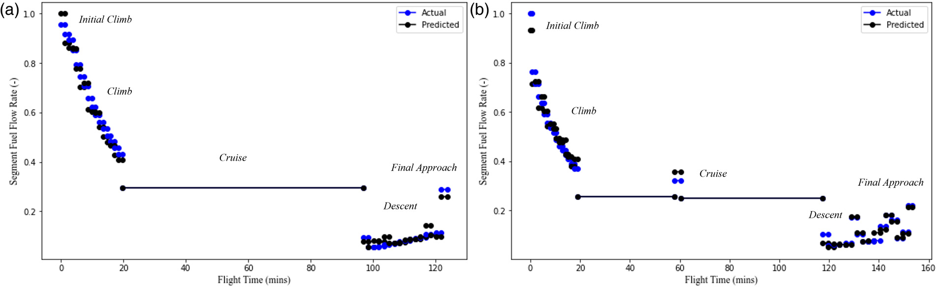
Table 4.
Final validation of calibrated model fuel-flow predictions for calibration and test datasets for B737-NG and B737-MAX models against actual flight data.
Hydrogen aircraft design
Liquid hydrogen tank
A cylindrical liquid hydrogen tank was sized for the hydrogen aircraft configurations using the required fuel combined with a target Gravimetric Index (GI), which is defined in Equation 4. The dimensions for the tank diameter and wall/insulation thickness were selected based on a detailed parametric analysis performed by Huete and Pilidis (2021), who designed a 100 m3 cylindrical tank for a short/medium-haul aircraft with a dormancy time of 24 h considering venting requirements and a maximum operating pressure of 404 kPa. The final tank design within this study resulted in a GI value of 0.66 (Huete and Pilidis, 2021), which is significantly greater than those observed in other studies, but can be seen as an optimistic value for EIS 2035–2050, where conservative estimates range from 0.2–0.35 (Mukhopadhya and Rutherford, 2022). To account for the uncertainty in GI values, and to analyse the influence of the GI on the outcomes of the current study, three GI values were used ranging from 0.33–0.66. A reduced external tank diameter of 3.8 metres, in contrast to the 4 metre diameter utilised by Huete and Pilidis (2021), was chosen to fit within the B737 fuselage – which has an effective diameter of 3.88 metres (Boeing, 2023).
Aircraft sizing
The LH2 aircraft sizing was performed using an iterative sizing loop, similar approach to that described in the author’s previous study (Gallagher et al., 2023a). The fuselage of each aircraft was extended by the length of the required LH2 tank in order to maintain a fixed design mission range of 2,950 NM, and a fixed payload and passenger capacity with respect to each respective conventional B737 configuration. A fixed payload and passenger capacity was required to maintain a consistent analysis of the real-world airline operations. An additional diversion of 250 NM was included in the sizing analysis to account for the reserve mission. Similarly to the study conducted by Mukhopadhya and Rutherford (2022), the wing-loading and thrust-to-MTOW ratio was maintained constant with respect to the original aircraft, where the propulsion mass was scaled in direct proportion to the thrust, and the sizing of the horizontal and vertical stabilisers was performed by maintaining a constant tail volume coefficient, which is outlined in Equation 5. S represents the reference area, c is the mean aerodynamic chord of the wing, and lH is the distance between the aircraft centre of gravity and the stabiliser centre of gravity, which was updated with each iteration to account for the LH2 tank. The aircraft component weights, which include the fuselage, wing, stabilisers and landing gear mass, were calculated for each iteration using correlations within SUAVE based on a combination of correlations from Shevell (1983); Lukaczyk et al. (2015).
Intercooling and recuperation
A preliminary IRE model was developed to assess the potential benefits available to LH2-powered aircraft. The IRE model was developed in NPSS based on data obtained from a recent compact heat exchanger design for a LH2 propulsion system (Patrao et al., 2024), where the current study aims to extend this IRE analysis to assess the impact of this technology when applied to a full range of airline operations. The NPSS IRE system illustrated in Figure 1b utilises the low-temperature LH2 fuel to reduce the air temperature before compression in the HPC as outlined in Equation 6, reducing the required HPC work, while heating the fuel to approximately 350 K. The hydrogen fuel is then used to recover heat from the core exhaust flow to elevate the fuel temperature to approximately 750 K, before delivering the fuel to the combustor with an increased enthalpy value (Patrao et al., 2024). As the current study is a scoping exercise, the heat transfer through the HEX ducts was not explicitly modelled, but instead correlated based on the data published by Patrao et al. (2024). Similar thermal management schemes have been analysed elsewhere, where inter-compressor cooling was found to have the greatest benefit with a ΔTSFC of −4.6%, followed by −2.6% and −1.7% for exhaust cooling and cooled cooling air (Görtz and Silberhorn, 2020).
The IRE model developed by Patrao et al. was for an increased technology level, utilising reduced fuel-flow and core mass-flow rates compared to the CFM56 and LEAP LH2 configurations. Therefore, to simulate an equivalent IRE for the current study, the heat transfer values obtained from Patrao et al. were scaled relative to the fuel-flow values at TOC, cruise, and RTO. The heat transfer values used for the current study’s models are outlined in Table 5, where the core mass flow of the CFM56 and LEAP NPSS models at TOC, RTO and cruise outlined in Table 5 were used to extrapolate the rate of heat transfer across the full range of engine operating points. To simulate the IRE operations within NPSS,
Table 5.
Intercooled-recuperated NPSS propulsion system data (Patrao et al., 2024).
The air-side pressure drop across the HEX ducts was calculated using Equation 7 (Kays and London, 1984), and applied to the NPSS models with a constraint of Δp < 9% to aid convergence across the full range of operating points. The LH2-IRE configuration resulted in an additional 326 kg per engine, with an extension of 1.04 metres to the propulsion system length (Patrao et al., 2024), which was implemented on each final LH2-IRE aircraft configuration outlined in the following section. Despite the simplified nature of the model, the TSFC reductions outlined in Table 5 yielded good agreement with the original TSFC reductions obtained from Patrao et al. (2024), where a maximum error of 0.8% pts was observed for the ΔTSFC values. Increased TSFCs were observed for low-throttle power points of the NPSS model, due to relatively low rates of heat transfer combined with the increased pressure drop across the HEX ducts. Further analysis with increased-fidelity models would be required to determine the validity of these results outside of the cruise, TOC and RTO operating points, which was outside the scope of this study.
Final aircraft designs
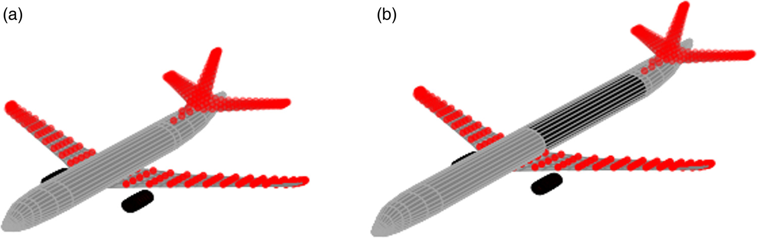
The final LH2 aircraft designs are presented in Table 6, where a B737-NG-LH2-0.33 configuration refers to an LH2 B737-800NG aircraft sized with a GI of 0.33, powered by a baseline LH2 engine (i.e., no intercooling/recuperation), whereas a B737-MAX-LH2-IRE-0.50 configuration refers to a LH2-powered B737-8200 aircraft sized with a GI of 0.50, with an intercooled and recuperated LH2 engine. The SAF-labelled aircraft refer to the conventional configurations (assuming identical fuel properties compared to Jet-A1), which are listed in Table 6 for reference. An example of the aircraft geometries generated within SUAVE are shown in Figures 8a and 8b, where the points highlighted in red represent the control points used in the VLM aerodynamic calculations, and the darker fuselage segment highlights the location and size of the LH2 fuel tank.
Table 6.
Final aircraft sizing parameters for B737-NG and B737-MAX models.
The influence of the GI on the LH2 aircraft designs can be observed in Table 6. With decreasing GI, there is an exponentially larger increase in MTOW, fuselage length, and fuel burn. This is due to the compounding effect of the GI – a larger tank mass results in increased fuel consumption, a longer fuel tank, and hence a larger and heavier fuselage and wing, which in turn results in greater fuel burn and a further extension to the LH2 tank length. However, the relationship is notably different for the B737-MAX aircraft compared to the less-efficient B737-NG aircraft, with significantly lower increases in the design mission fuel burn, and hence the fuselage length, with decreasing GI. This is due to the increased fuel efficiency of the B737-MAX aircraft, which consumed 12% less fuel than the B737-NG aircraft on its design mission for the conventional (SAF) configuration. With increasing fuel-efficiency, the relative impact of the in-flight performance penalties associated with LH2-powered aircraft are reduced, and therefore the influence of the GI on the aircraft performance is less significant. This characteristic means that it is particularly important to have accurate fuel burn models for future aircraft when conducting studies on LH2 operations, and for analysing the impact of GI on LH2-aircraft in general. The effect of the IRE model is also observed in Table 6, where despite yielding similar MTOW values compared to the standard LH2-0.50 configurations, the design fuel burn was reduced by 4.6% and 4.7% for the B737-NG and B737-MAX aircraft, respectively.
Hydrogen and SAF operations
Operation schedule
The operation schedule selected for the LH2-SAF case study consisted of the flights to and from any Irish airports, i.e., Dublin, Belfast, Cork, Shannon and Knock, within the complete flight database. The final schedule consisted of 257 B737-NG flights, where the average mission range of these 257 flights was 659 NM. Due to the relative lack of B737-MAX operational data, 25% of the B737-NG flights were modelled using the B737-MAX aircraft model to simulate the flight schedule, based on the fleet split of the airline, which consisted of 411 B737-NG to 137 B737-MAX aircraft at the time of writing (Flightradar24, 2024).
Well-to-Tank energy efficiency
The P2L fuels analysed in this study include SAF-DAC, produced via synthesis of green hydrogen with carbon sequestered through DAC processes, and green LH2, produced via electrolysis of water followed by liquefaction to −253°C, where the electricity source is assumed to be 100% renewable electricity for each fuel. SAF produced via Fischer-Tropsch (FT) and Alcohol-To-Jet (ATJ) processes, which are American Society for Testing and Materials (ASTM) approved SAF pathways using biogenic feedstocks, were also included in the analysis for reference as near-term, low-carbon SAF solutions (Grim et al., 2022). All SAF and LH2 production was assumed to be zero-carbon or net-zero due to the low reported CI values (Grim et al., 2022), and hence analysis on emissions was not considered in the current study. Furthermore, a lifecycle assessment of each fuel was outside of the scope of this study, however detailed life-cycle impact studies are presented here for reference (Bicer and Dincer, 2017; Micheli et al., 2022; Weidner et al., 2023)
The Well-to-Tank (WtT) efficiency describes the energy efficiency of the production process for each fuel (i.e., the required energy input in MJ per MJ of fuel produced). The WtT efficiencies for the SAF pathways outlined in Table 7 were selected based on a detailed investigation and analysis of SAF production processes, where SAF-DAC represents an average of three DAC processes of varying production efficiency (Grim et al., 2022). The LH2 production efficiency was estimated using an electrolysis efficiency of 75%, liquefaction efficiency of 75%, and distribution efficiency of 99% (Tashie-Lewis and Nnabuife, 2021), resulting in a final WtT efficiency of 55.7%. This figure is closely aligned with values reported in similar studies, where LH2 WtT efficiencies ranged from 56–58% (Clean Sky 2 JU and FCH 2 JU, 2020; Mukhopadhya and Rutherford, 2022). The WtT efficiencies for each fuel are listed in Table 7.
Table 7.
Well-to-Tank efficiencies for each fuel (Tashie-Lewis and Nnabuife, 2021; Grim et al., 2022).
| Fuel Type | SAF-DAC | SAF-ATJ | SAF-FT | Green LH2 |
|---|---|---|---|---|
| Well-to-Tank Efficiency | 30.3% | 39.3% | 43.6% | 55.7% |
Results and discussion
Tank-to-wake analysis
The operation schedule outlined in the previous section was simulated to obtain the fuel burn of each flight for each aircraft configuration, and each aircraft configuration was analysed in terms of its Tank-to-Wake (TtW) energy consumption (i.e., the energy contained within the fuel burned during flight), which was calculated by multiplying the fuel burn by the LHV as outlined in Equation 8.
B737-NG
A sample flight with a mission range of approximately 1,500 NM was selected from the operation schedule to analyse the TtW performance of each aircraft, which is illustrated in Figure 9. These results clearly shows the detrimental impact of a low GI value on the in-flight energy performance, as the LH2-0.33 configuration yielded a 48.4% increase in energy for the 1,500 NM flight when compared to the SAF configuration, largely due to the significant difference in TOW value, which was 43% greater than the SAF aircraft. This resulted in a significantly higher rate of energy consumption during each flight phase, especially for the climb phase due to the increased induced drag. However, the compounding effect of the GI value on energy performance is observed in the results of the LH2-0.50 and LH2-0.66 configurations, which yielded more moderate performance penalties of 19.8% and 12.1%, respectively. The LH2-IRE configuration with a GI value of 0.50 resulted in a 14.4% performance penalty compared to the SAF aircraft, highlighting the potential of an LH2-IRE as an enabling technology to bridge the in-flight performance gap between LH2 and SAF.
Figure 9.
Tank-to-Wake energy performance of B737-NG LH2 and SAF configurations for a 1,500 NM mission.
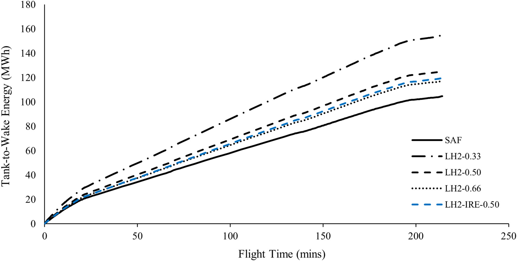
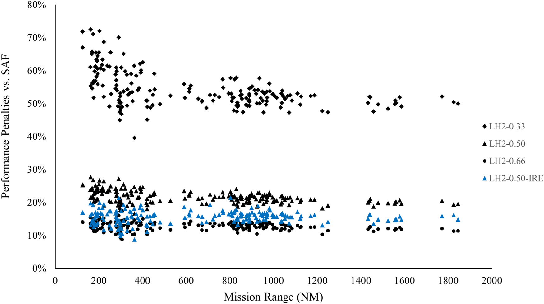
Figure 10 shows the TtW energy performance penalties, i.e. the relative increase of in-flight energy consumption, for each LH2 aircraft configuration when compared to the conventional SAF aircraft for the full range of B737-NG operations. An interesting trend is observed for the LH2-0.33 aircraft, which yielded significantly increased performance penalties for missions with a range <500 NM, reaching penalties >70%. This was due to the higher Operating Empty Weight (OEW) coupled with lower fuel weight savings for short-range missions associated with the lower mass of the LH2 compared to SAF. A similar, albeit much less exaggerated, trend was observed for the three remaining LH2 candidates, with slightly increasing relative performance penalties towards short-range missions, reaching a maximum of 27.7% and 16.0% for the LH2-0.50 and LH2-0.66 aircraft, respectively.
B737-MAX
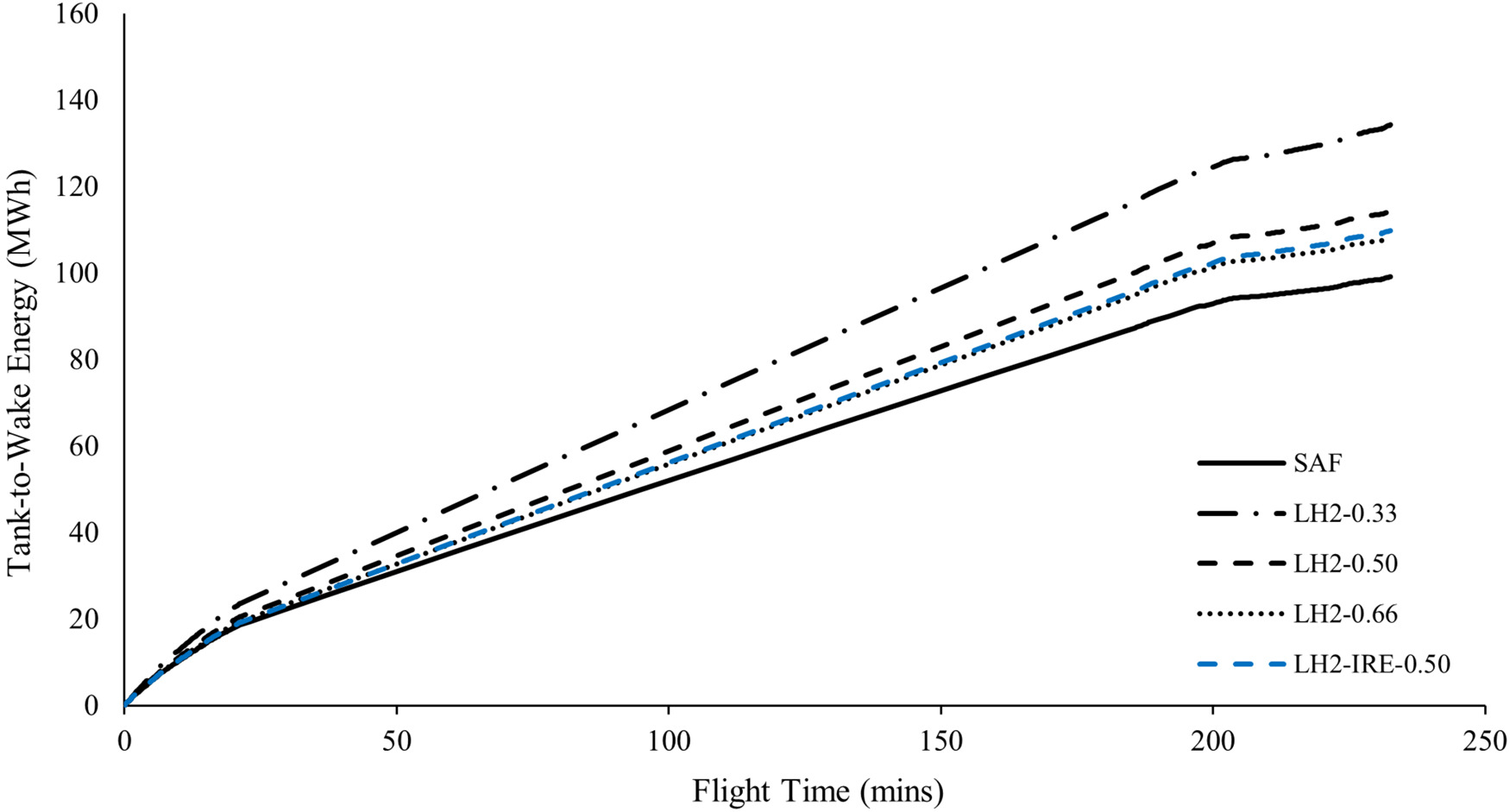
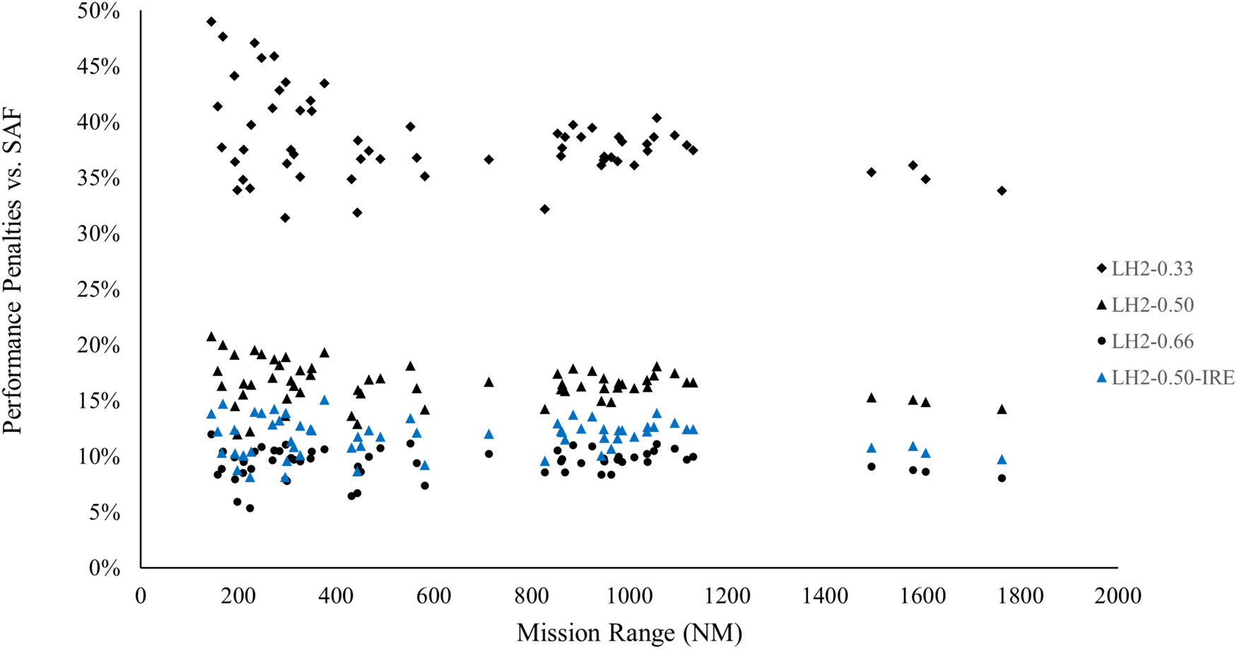
Similarly to the previous section, a flight with a mission range of approximately 1,500 NM was selected for a TtW analysis of the B737-MAX aircraft configurations, where the results are illustrated in Figure 11. The reduced influence of the GI value for the more fuel-efficient B737-MAX aircraft is clearly visible, as the LH2-0.33 configuration resulted in just a 35.5% increase in the TtW energy consumption compared to SAF, which reduced to 15.3% and 9.1% for the LH2-0.50 and LH2-0.66 configurations, respectively, while the LH2-IRE candidate resulted in similar relative performance improvements shown in the previous section, with the performance penalty reduced to 10.8% vs. the SAF B737-MAX aircraft. The performance penalties for the full range of operations are shown in Figure 12, where the overall reduction in performance penalties for the B737-MAX aircraft are observed, and similar trends resulted regarding the increased performance penalties for short-range missions, reaching maximum values of 49.0%, 20.8%, 12.0% for the LH2-0.33, LH2-0.50, and LH2-0.66 configurations, respectively.
Well-to-Wake analysis
The Well-to-Wake (WtW) energy was calculated by dividing the TtW energy in Equation 8, by the WtT efficiency of each fuel previously outlined in Table 7, and the fleet-wide WtW energy results for the three SAF candidates and three LH2 configurations are reported in Table 8 for both aircraft and the total fleet. SAF-DAC was found to be significantly more energy intensive than all LH2 aircraft, requiring 43.8% more energy than the LH2-0.33 aircraft for the total fleet operations. SAF-ATJ resulted in 4.9% lower energy consumption than the LH2-0.33 configuration for the total fleet, but was 3.1% more energy intensive when compared to the B737-MAX LH2-0.33 missions, indicating that this may be a worse-performing option than LH2 for modern aircraft. SAF-FT yielded energy reductions of 14.3% vs. the total fleet of LH2-0.33 aircraft, but was outperformed by both the LH2-0.50 and LH2-0.66 aircraft with 6.5% and 14.2% higher energy consumption, respectively.
Table 8.
Fleet-wide energy and cost results for LH2 vs. SAF operations.
Furthermore, the minimum cost of the renewable electricity required to power these operations was estimated using the Levelised Cost Of Electricity (LCOE) of Europe’s North Sea off-shore wind power hub, which is reported to deliver renewable wind energy at a break-even cost of €40/MWh post-2030 (Ruijgrok et al., 2019). Analysing the LCOE was preferred due to the assumption that these future fuels will be produced using 100% electricity, and due to the fact that estimated future fuel costs for LH2 and SAF are extremely uncertain – however, it is certain that P2L SAF would be more expensive than green LH2 due to the additional capital and process requirements. Although the LH2-0.50 and LH2-0.66 fleet outperformed all SAF candidates in terms of WtW energy performance and LCOE, these results must be considered in the context of the infrastructural challenges, aircraft development cost, and increased complexity of LH2 aircraft operations, which was outside of the scope of this study. As a result, near-term SAF options such as ATJ and FT may be more desirable if sufficient feedstock is available. However, it is clear that SAF-DAC operations would introduce significantly larger fuel costs — up to €617,840 for 257 flights compared to LH2-0.66 – which may outweigh the benefits of maintaining a drop-in fuel solution.
Intercooling-recuperation analysis
The fleet-wide energy results of the LH2 and LH2-IRE configurations are presented in Table 9, where only a GI value of 0.50 was analysed as a simplifying measure. The LH2-IRE configuration for the B737-NG and B737-MAX aircraft resulted in a 4.6% and 3.9% reduction in energy compared to the baseline LH2 configurations, respectively with a total fleet-wide energy reduction of 4.4%. Although these reductions may seem relatively insignificant, when applied to a full operating schedule, significant savings in both energy and cost could be obtained – over 1 GWh and €46 k for 257 flights – reducing the strain on renewable electricity resources, and increasing the economic viability of LH2 aircraft. The results of the IRE model further strengthens the case for LH2-powered aircraft, and represents a potential enabling technology for zero-carbon aviation.
Table 9.
Fleet-wide energy and cost results for LH2 vs. LH2-IRE aircraft model.
Conclusions
An operational case study was performed to evaluate the fleet-wide energy performance of LH2-powered vs. SAF-powered B737-NG and B737-MAX aircraft, for a large short-haul European airline. The conventional SAF aircraft, alongside the developed LH2 and LH2-IRE configurations were simulated over a full day of airline operations to and from the island of Ireland (257 flights) low-fidelity aircraft modelling methods with exceptional accuracy. The performance of each aircraft was comparatively evaluated in terms of the TtW and WtW energy consumption, along with the renewable electricity cost required to power these operations.
It was found that despite higher in-flight energy penalties for the LH2 candidates, the LH2-0.50 and LH2-0.66 fleets outperformed all SAF pathways analysed. SAF-DAC was found to be particularly energy intensive, consuming 44% more energy than the lowest-performance LH2-0.33 aircraft. Near-term SAF-ATJ and SAF-FT options were found to be viable in comparison to LH2, yielding maximum fleet-wide WtW energy penalties of 27% and 14%, respectively, however these fuels lack the long-term sustainability of P2L fuels as discussed in previous sections. The LH2-IRE configuration was found to have a significant benefit for LH2 aircraft performance, reducing the total fleet-wide energy consumption by 4.4%. These results aim to provide a realistic estimate of the real-world energy performance of fleet operations for LH2 and SAF aircraft, where the results may be used to further analyse the trade-offs associated with infrastructure requirements, aircraft design, alongside operating cost and total energy consumption.
This study is part of a wider project in evaluating the feasibility of hydrogen-powered aircraft against SAF-powered aircraft, which aims to assess the trends in performance from current, state-of-the-art technologies, towards advanced aircraft with entry-into-service of 2035–2050. Increased fuel efficiency (and LH2 tank GI) reduces the relative impact of in-flight performance penalties associated with large LH2 fuel tanks, which was observed in the transition from the B737-NG to the B737-MAX aircraft. Future studies will incorporate an advanced B737-type aircraft, where the performance trends will once again be evaluated over a representative operating schedule to assess the real-world impact in terms of energy and cost, helping to identify the optimum future aircraft and fuel solutions in terms of minimum operating cost and energy consumption. These analyses aim to inform data-driven policy incentives to provide the best chance for an economically sustainable decarbonisation pathway, encouraging the transition to net-zero aviation while minimising the strain on renewable electricity resources.
Nomenclature
ADS-B
Automatic Dependent Surveillance-Broadcast
ASTM
American Society for Testing and Materials
ATJ
Alcohol-To-Jet
DAC
Direct Air Capture
FT
Fischer-Tropsch
GI
Gravimetric Index
HEX
Heat Exchanger
IC
Intercooler
IRE
Intercooled-Recuperated Engine
LH2
Liquid Hydrogen
LHV
Lower Heating Value
MTOW
Maximum Take-Off Weight
NM
Nautical Miles
NPSS
Numerical Propulsion System Simulation
OEW
Operating Empty Weight
P2L
Power-to-Liquid
RC
Recuperator
RTO
Rolling Take-Off
SAF
Sustainable Aviation Fuel
SLS
Sea-Level Static
SLSQP
Sequential Least-Squares Quadratic Programming
SUAVE
Stanford University Aerospace Vehicle Environment
TOC
Top-Of-Climb
TOW
Take-Off Weight
TSFC
Thrust Specific Fuel Consumption:
TtW
Tank-to-Wake
QAR
Quick-Access-Recorder
VLM
Vortex-Lattice Method
WtT
Well-to-Tank
WtW
Well-to-Wake
CD
Drag Coefficient
Dh
Hydraulic Diameter, m
E
Energy, MWh
G
Mass Flux, kg/m2
Hz
Frequency, 1/s
Lx
HEX Length, m
Heat Transfer Rate, kW
S
Reference Area, m2
T
Temperature, K
V
Volume Coefficient
cp
Specific Heat Capacity, kJ/kg·K
lh
Moment Length, m
m
Mass, kg
p
Pressure, Pa
ρ
Density, kg/m3
σ
Flow/Frontal HEX Area