Introduction

Modern propulsion turbomachinery design features high loading and compactness. Highly loaded blades often have thick boundary layer on blade suction surface around the blade trailing edge region even at their design operating point. As a consequence, the thick wakes will not be readily mixed out fully with the flow field within the blade passages of the immediate downstream blade row, and thus can reach farther downstream blade rows. Compact designs with reduced axial dimensions exacerbate this situation. The wakes from non-adjacent upstream blade rows have profound effect on turbomachinery aerodynamics and aeroelasticity. It is essential to capture the associated flow features in an efficient manner so that their effects can be properly assessed in a routine design environment.

The efficient analysis of rotor-rotor/stator-stator interference using the nonlinear harmonic method by He et al. (2002) probably represents the earliest such an effort. The separate solution of each harmonic allows a straightforward application of the nonlinear harmonic method for analyzing wakes from non-adjacent blade rows, as passage harmonics involved in a rotor-rotor or stator-stator interaction can be considered time harmonics with zero frequency. The nonlinear harmonic method is further extended and generalized by Vilmin et al. (2013) for arbitrary number of rows of turbomachinery. The extended nonlinear harmonic method is now available in the commercial software of FINE/TURBO and it has been advertised as the rank-N nonlinear harmonic method(Teixeira, 2020) or the limitless nonlinear harmonic method (Baux, 2021).

Using the harmonic balance method to capture wakes from non-adjacent blade rows is much more difficult, as the solution of all harmonics is tightly coupled in the method. To enable the harmonic balance method to capture disturbances from blade rows which are stationary with respect to each other, Subramanian et al. (2013) proposed the all blade row algorithm, which introduces small fictitious rotation rates to originally stationary blade rows. This approach requires to retain a large number of frequencies in a blade row and diminishes the computational saving of the harmonic balance method. Furthermore, fictitious rotation rates will inevitably introduce solution errors. Another effort is the development of the harmonic set approach (Frey et al., 2014), which is based upon the nonlinear frequency domain method (Mcmullen et al., 2006). The harmonic set approach was originally proposed to handle unsteady flows with multiple fundamental frequencies by grouping unsteady flow components according to their fundamental frequencies. The grouping of frequency components and their separate time sampling and residual calculation lend the method the capability of calculating wakes from non-adjacent blade rows (Junge et al., 2015). It should be noted that the harmonic set approach has its own inherent limitations: it cannot consider the nonlinear interactions between different groups of harmonics and it also introduces a certain level of programming complexities.

A coupled time and passage spectral method (Wang et al., 2021) has been proposed for efficient analysis of wakes from non-adjacent upstream blade rows. The coupled time and passage spectral method is a natural and simple extension of the existing time domain harmonic balance method (Hall et al., 2002). Same as the harmonic balance method, it uses a truncated Fourier series to approximate temporally and spatially periodic flows. With the use of a phase shift boundary condition, one blade passage per blade row can be used for an analysis. The coupled time and passage spectral method circumvents some limitations of the harmonic balance method: it can accommodate situations where (1) the time averaged flow varies from passage to passage in a blade row, (2) there exist unsteady flow components which have the same frequency but different inter blade phase angles. This is achieved by including inter blade phase angle and passage index in a truncated Fourier series, which is essentially a coupled temporal and spatial Fourier representation.

The coupled time and passage spectral method is expected to provide considerable computational cost saving in contrast to the harmonic balance method with a domain consisting of multiple blade passages. To achieve this, the required extra time and space harmonics have to be very limited. Furthermore, it is vitally important to establish some rules for specifying those extra time and space harmonics. Junge et al. (2015) proposed a posterior iterative approach to establish the time and space modes which have to be retained in an analysis. Temporal and spatial Fourier transforms are performed at a rotor-stator interface to extract the amplitudes of axial velocity of all available temporal and spatial modes. For a given time mode, the axial velocity amplitude often has its peak around the zero nodal diameter, and reduces with the increase of the absolute value of a circumferential nodal diameter. It recommends that only modes which have significant axial velocity amplitude be retained in an analysis. In view of this, it is very desired to establish a priori rules. The aim of this study is to establish rules for specifying extra time and space harmonics for a coupled time and passage spectral analysis by analyzing results from a harmonic balance analysis using multiple blade passages for a two-stage transonic fan. Then the validity of the proposed rules will be demonstrated and refined through a series of coupled time and passage spectral analyses for the same configuration.

Coupled time and passage spectral method

The coupled temporal and spatial Fourier series of the coupled time and passage spectral method is given by

where U¯ is the time and passage averaged flow variable, Cn is the complex Fourier coefficient, ℜ indicates the real part of a complex number, j is the blade passage index, t is time, x is the spatial coordinate, N is the number of harmonics being retained in an analysis, ωn and δn are the angular frequency and inter blade phase angle of the nth harmonic. The inclusion of the passage index j and inter blade phase angle δn in Equation 1 can differentiate harmonics with the same frequency but different inter blade phase angles. Thus, harmonics with the same frequency but different inter blade phase angles can be accommodated in one series without degenerating the involved Fourier transform matrix. Furthermore, zero frequency harmonic, which represents a passage harmonic, can also be included in Equation 1.

To implement the coupled time and passage spectral method in an existing harmonic balance solver, a few modifications are required: (1) the first is to include the contribution of inter blade phase angle in a phase calculation (from ωnt to ωnt+jδn); (2) time sampling has to be performed over multiple blade passages of a blade row to ensure a Fourier transform matrix having a small condition number. The time and passage sampling can be achieved through an initial passage and time oversampling followed by the modified Gram–Schmidt process to choose the time and passage instants which give the most orthogonal 2N + 1 row vectors of the inverse Fourier transform matrix.

The coupled time and passage sampling gives the wrong impression that multiple blade passages of a blade row have to be used in an analysis. The proper interpretation of the time and passage sampling is that flow fields at different time instants and different blade passages are solved. These flow fields are linked through the coupled time and space spectral operator. More than one time instants can be chosen from one blade passage, while there might be passages where no flow solutions are sought directly.

To analyze wakes from a non-adjacent upstream blade row, it is essential to extract the wake components at a rotor-stator interface and pass it to the downstream blade row. The wake extracting and relaying process has to be performed for the same wake at a few downstream rotor-stator interfaces. The time and space mode decomposition and match method (Wang and Huang, 2017) is used to facilitate such an operation.

Wake propagation and mode scattering

Wakes of a blade row can be considered steady in the frame of reference attached to that blade row. However, the same wakes are unsteady when being viewed in the frame of reference which rotates relative to blades generating them. The wakes will interact with local flow field and generate scattered modes when they propagate downstream. It is essential to understand the mechanism of wake propagation and mode scattering when analyzing blade row interaction unsteady flows in a multi-stage environment.

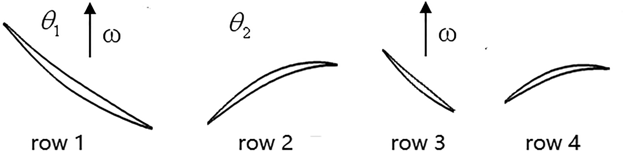
Without loss of generality, we consider a two-stage configuration (Figure 1) with blade counts of N1, N2, N3 and N4 for the first, second, third and fourth blade rows. The first and third blade rows rotate in the positive circumferential coordinate direction at the angular speed of ω, and the second and fourth rows are stationary. A wake component of row 1 at the interface between the first and second rows can be represented in complex number as

Figure 1.

A two-stage configuration for the illustration of wake propagation and mode scattering.

where Cn1 is the complex amplitude of the wake component, n is a positive integer, θ1 is the circumferential coordinate of row 1. When being viewed in the frame of reference attached to the second blade row, the wake component is in the following complex form:

where θ2 is the circumferential coordinate in the frame of reference attached to the second blade row. The relationship between θ1 and θ2 is given by

From Equation 3, we can see that the wake component varies with time, which means it is unsteady in the frame of reference attached to the second blade row. The interaction of the wake component with local flow fields in the domain of the second blade row generates scattered modes, namely,

where m is an integer which can be negative, zero or positive. Note that the amplitude of the wake component changes after its interaction with local flow field. When being viewed in the frame of reference attached to the third blade row, the wake component takes the following complex form:

The wake component interacting with the local flow field of row 3 generates scattered modes, which can be expressed as follows

Similar to m, l is an integer which can be negative, zero and positive. Coming to the frame of reference attached to row 4, the wake component of Equation 7 takes the following complex form:

In theory, n can range from 1 to +∞, m and l can range from −∞ to +∞. However, it is impractical and unnecessary to resolve all modes, as a limited number of modes are expected to be significant. Though including many modes can provide a more accurate solution, it will inevitably incur more computational cost. Therefore, to efficiently resolve the blade wakes of the first and second blade rows in the domains of their downstream blade rows, it is vitally important to set n, m and l to proper values.

To resolve the wake in the domain of the second blade row, quite often about 6 harmonics are needed, that is to set n=1,…,6, as established in a previous study (Wang and Huang, 2017). To resolve the wake in the domain of the third blade row, one needs to set values for both n and m. The general wisdom is that the significance of modes decreases with the increase of |n| and |m|. If the wake is not fully dissipated at the exit of the third blade row, then there is a need to resolve it in the domain of the fourth blade row if it exists. Choosing the appropriate values of n and m for the third blade row and the fourth row if applicable a priori is a challenge which will be investigated in this study.

Methodologies

Both the harmonic balance method and the coupled time and passage spectral method have been implemented in an existing in-house flow solver-TurboXD. The flow solver solves the Reynolds averaged Navier–Stokes equation in a cylindrical coordinate system attached to blade rows under consideration, but solution variables are those in a stationary frame of reference. The eddy viscosity is calculated using the one equation Spalart Allmaras model (Spalart and Allmaras, 1992). The partial differential equations are solved in the framework of the cell centered finite volume method. The convective fluxes are calculated using the well known Jameson–Schmidt–Turkel scheme (Jameson et al., 1981) with artificial dissipation being scaled by spectral radius of the flux Jacobian matrix. The first order spatial derivatives of flow quantities required for physical dissipation calculation are obtained at cell centers using the Gauss’s theorem. Pseudo-time integration is accomplished using a hybrid explicit and implicit method: the 5-stage Runge Kutta method and the Lower-Upper Symmetric Gauss–Seidel(LU-SGS) (Yoon and Jameson, 1988). The LU-SGS method is used as a residual smoother at each stage of the 5-stage Runge Kutta method to achieve convergence speedup by allowing for a Courant number up to hundreds even thousands. For a harmonic balance analysis or a coupled time and passage spectral analysis, the implicit treatment of the time spectral source term is different from the rest of the equations to reduce implementation complexity. The time spectral source term is implicitly integrated using a one-step Gauss–Seidel method, while the rest is integrated using the LU-SGS scheme (Huang et al., 2018). A V-type multigrid is also available for convergence acceleration.

Test case introduction

To establish the rules for specifying extra time and space harmonics for a coupled time and space spectral analysis, a two-stage transonic fan is used as the test vehicle. Though it does not represent the state of art design, the wakes of the first blade row can reach the fourth blade row and the wakes of the second blade can reach the fourth blade row as revealed in previous investigations. Thus the flow fields within the fan possess required features for this study. The fan has no inlet guide vane, thus there are four blade rows in total. The blade counts are 28, 46, 60 and 59 for the first to fourth rows, respectively. It can be seen that the blade counts are generic, as the greatest common factor of blade counts is quite small. This implies that rules established in the study will be generic.

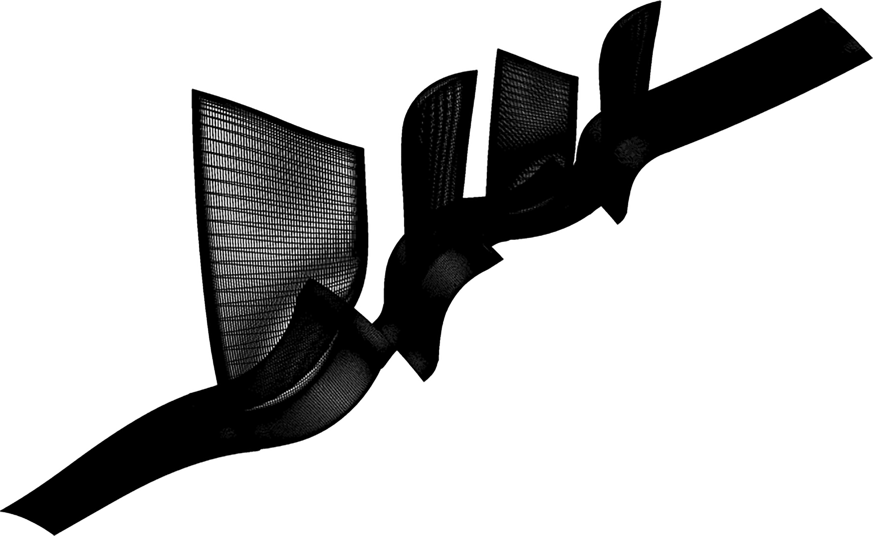
Each blade passage is meshed using an H-type topology. There are 61 and 73 grid points in the circumferential and radial directions and about 110 grid points on a blade surface in the chord-wise direction. The average number of grid points for each blade passage is about 750,000, resulting in about 3 million grid points for a domain consisting of one blade passage per blade row. The isometric view of the mesh on the hub and blade surfaces is presented in Figure 2.

Figure 2.

Isometric view of the mesh on the hub and blade surfaces.

All the analyses to be presented involve five types of boundaries. At the domain inlet, uniform total pressure (101,325 Pa) and total temperature (288.15 K) and flow angle (axial) are specified. At the domain outlet, an area averaged static pressure of 2.2e5 Pa is specified. On blade surfaces, hub and shroud surfaces, a slip wall boundary condition is used, together with a wall function for calculating wall shear stress (Denton, 1992), to avoid resolving the viscous sublayer. A phase shift boundary condition is applied at the lateral periodic boundaries for either a harmonic balance analysis or a coupled time and passage spectral analysis. The interface treatment based upon time and space mode decomposition and match (Wang and Huang, 2017) is used for an inter blade row interface.

Harmonic balance analysis for mode identification

Two harmonic balance analyses were conducted to analyze the unsteady flow field within the two-stage fan. One analysis (designated as HB-1) used a computational domain consisting of one blade passage for each blade row. This case will demonstrate the limitation of the harmonic balance method in capturing wakes from non-adjacent blade rows. As will be shown later, the wakes of the first blade row cannot be captured in the passages of the third blade row and the wakes of the second blade row cannot be captured in the passages of the fourth blade row. The other analysis (designated as HB-15) used a computational domain consisting of multiple blade passages for the third blade row and one blade passage for other three rows. With the use of a domain consisting of multiple blade passages for the third blade row, the wakes of the first blade row can be captured in the passages of the third blade row.

The blade counts of the first and third blade rows (28 and 60) have the greatest common factor of 4, thus to fully capture the wakes of the first blade row, the third row has to use a domain of one fourth of the annulus (15 blade passages). To fully resolve the wakes of the second blade row in the passages of the fourth blade row, a whole annulus domain has to be used for the fourth blade row(the greatest common factor of the blade counts of the second and fourth rows (46 and 59) is 1), for which the requirement of computing resources is prohibitive. Therefore, the resolution of the wakes from the second blade row in the passages of the fourth blade row is not considered in the second harmonic balance analysis.

In the two harmonic balance analyses, six harmonics are used to resolve a wake and three harmonics are used to resolve a downstream nonuniform potential field. Therefore, three, nine, nine and six harmonics are retained in the domains of the first, second, third and fourth blade rows, respectively. The specification of frequencies and inter blade phase angles (IBPA) of each row is provided in Table 1. Note the inter blade phase angles of the third blade row for the HB-15 analysis are actually inter sector phase angles, as they are calculated based upon the domain sector, which amounts to one fourth of the whole annulus for the third blade row. The sign of inter blade phase angle is defined as such: in a frame of reference attached to a blade under consideration, if a disturbance travels at the shaft rotation direction, then the sign of the corresponding inter blade phase angle is positive. According to the time and space mode decomposition and match method, there are 46 time and space modes at each rotor-stator interface for the first analysis. The number of time and space modes at the second rotor-stator interface for the HB-15 analysis is 124, which is much more than that of other interfaces.

Figure 3 shows the reconstructed instantaneous entropy at 90% blade span. For the HB-1 analysis, marked entropy discontinuity can be observed at the interface between the second blade row and the third blade row and that between the third blade row and the fourth blade row. The flow discontinuity demonstrates the limitation of the harmonic balance method in capturing wakes from non-adjacent blade rows.

Figure 3.

Reconstructed instantaneous entropy at 90% blade span.

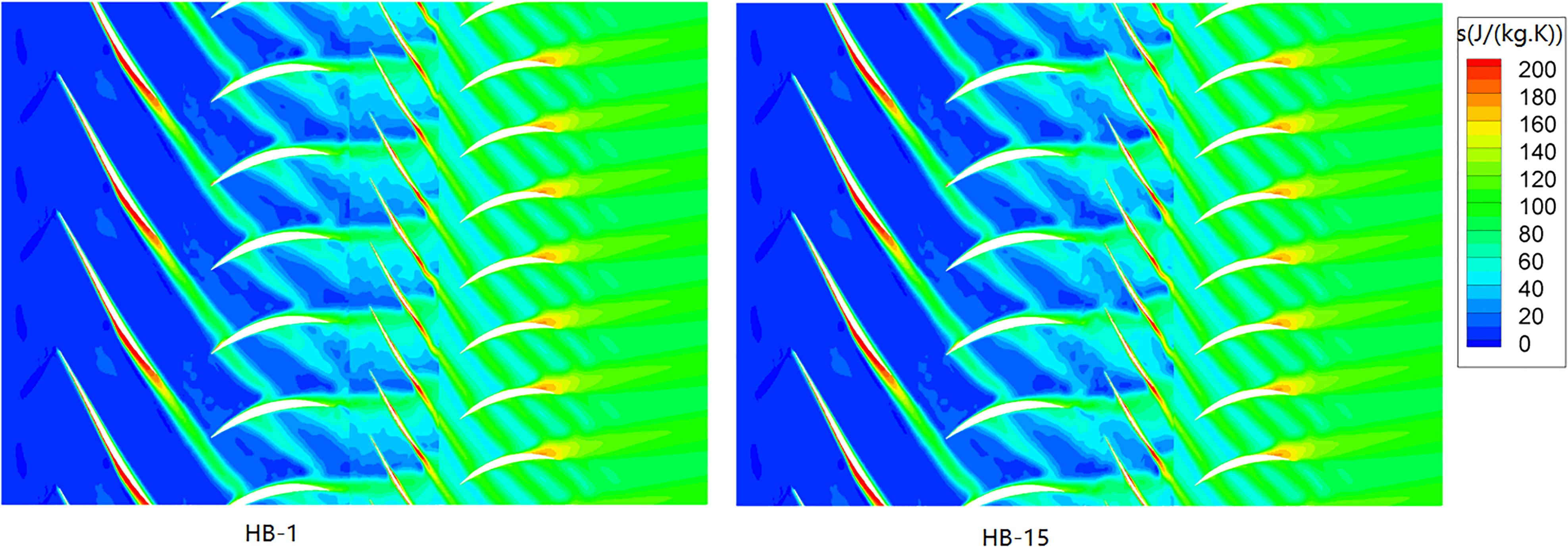
From Figure 3, it can also be seen clearly that the wakes of the first row propagate smoothly through the interface between the first row and the second row. There is no loss of resolution of the wakes in the domain of the second blade row. The wakes are not fully dissipated in the passages of the second row and they propagate further through the interface between the second row and the third row. With the HB-15 analysis, the entropy is continuous at the second rotor-stator interface and there is no loss of resolution on the downstream side of the interface. Note there is also discontinuity at the interface between the third and fourth blade rows for the HB-15 analysis, as one blade passage is used for the fourth blade row and the wakes of the second row are not intended to be captured in the passages of the fourth blade row.

As fifteen blade passages are used for the domain of the third blade row in the HB-15 analysis, the time averaged flow field can accommodate eight spatial modes and unsteady flow of a given frequency can accommodate fifteen spatial modes, according to the Nyquist theorem. The local mode index of the spatial modes for the time averaged flow ranges from 0 to 7. The index 0 pertains to the time and passage averaged flow field. The local mode index of the spatial modes for unsteady flow of a given frequency ranges from 1 to 15. The local mode index is established on a domain which is one fourth of the whole annulus, thus the nodal diameter of a spatial mode is 4 times that of a corresponding local mode index plus the nodal diameter corresponding to the inter blade phase angle being imposed for that frequency component. The difference in the local mode index range for the time averaged flow and unsteady flows is due to the fact that the time averaged circumferentially non-uniform flow is fixed in space and has no direction and non-uniform unsteady flows with a non-zero diameter represent traveling waves and can travel in both directions.

In the following, the spatial modes for both time averaged and unsteady flows are extracted and presented. The spatial modes are extracted through discrete Fourier transform for all possible mode indices. First, the spatial modes for the time averaged static pressure, static temperature and turbulence quantity are shown in Figure 4. The spatial mode with the biggest amplitude has an index of 7 corresponding to a nodal diameter of 28. This corresponds to the blade count of the first row, revealing that the passage variation of time averaged flow is truly due to the influence of the first row. The spatial mode with index 1 has a small region of visible amplitude. This corresponds to a nodal diameter of 4. Though not straightforward, it can be found that this is from the second harmonic of the row 1 wake: 60−28*2 = 4. Other spatial modes have negligible amplitudes. In summary, to resolve the passage variation of time averaged flows, it suffices to include the first harmonic of row 1 wakes. Referring to Equation 6, this corresponds to setting m = 0 and n = 1.

Figure 4.

Amplitudes of all spatial modes of the time averaged static pressure (left), static temperature (middle) and turbulence quantity (right).

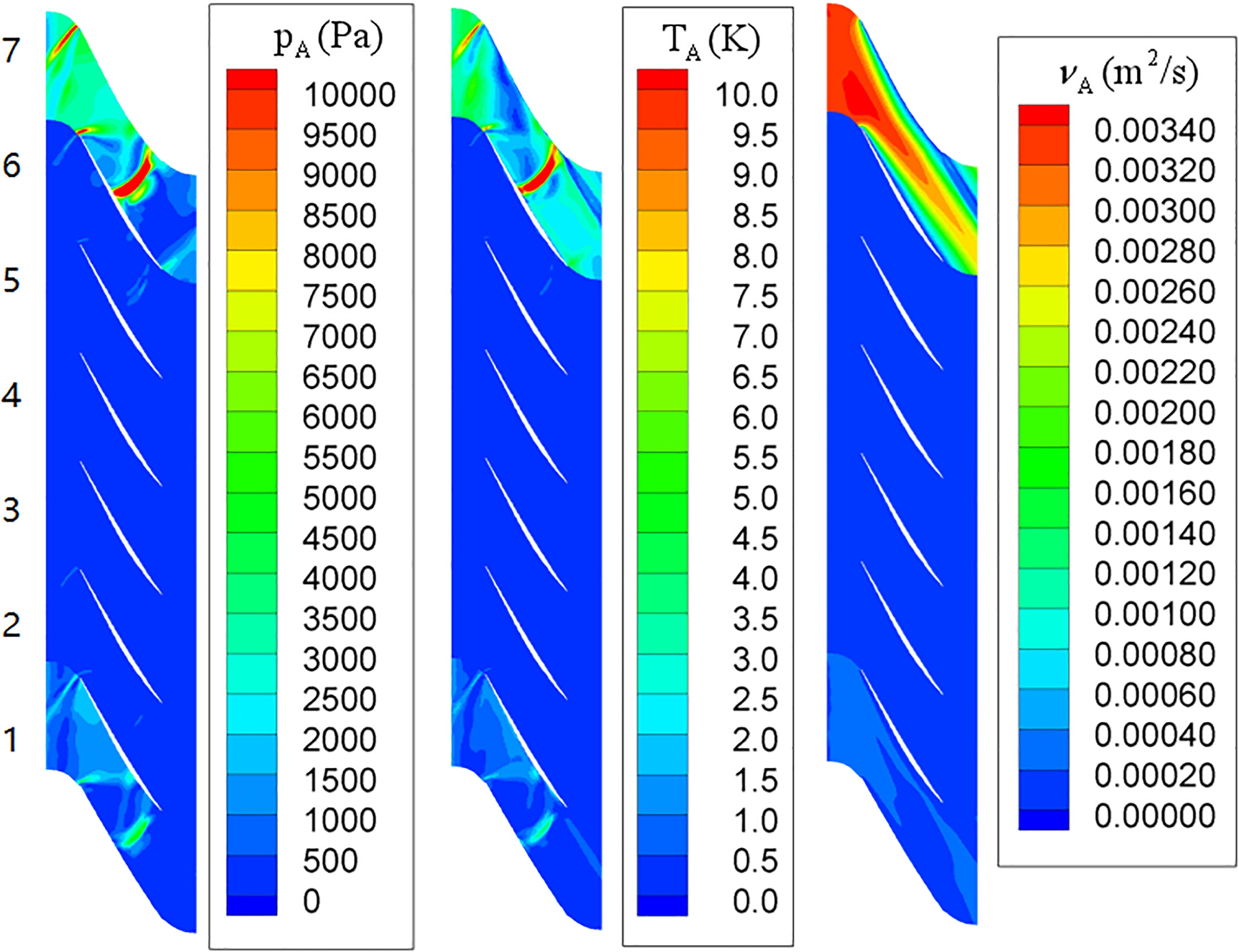
Now we look at the spatial modes of static pressure, static temperature and turbulence quantity for three different frequencies: the upstream stator blade passage frequency (1SBF), its second harmonic (2SBF) and third harmonic (3SBF), as shown in Figure 5. With the increase of unsteady flow frequency, the maximum amplitude of static pressure, static temperature and turbulence quantity reduces significantly. For each frequency component, be it static pressure, static temperature or turbulence quantity, there are very few limited spatial modes which are significant. Those significant modes only need to be retained in an analysis.

Figure 5.

Amplitudes of all spatial modes of unsteady static pressure, static temperature and turbulence quantity with stator blade passage frequency (1SBF), its second harmonic (2SBF) and third harmonic (3SBF).

For the first harmonic of static pressure, there are two dominant modes: the one with the local mode index of 8 and the one with the local mode index of 15. For the first harmonic, an inter blade phase angle corresponding to the upstream stator wake is imposed in the analysis. The nodal diameter of the wake is 46. Therefore, the local mode index of 8 has a nodal diameter of 18 (46 + 8*4 = 46 − 28 + 60 → 46 − 28), which reveals that this spatial mode results from the first harmonic of row 1 wake. Referring to Equation 6, this corresponds to setting n = 1 and m =  − 1 (Note the signs of m and n are reversed when the frequency of unsteadiness is negative). It can be seen from Figure 5 that this mode is not fully mixed out within the blade passages of row 3 and its amplitude is significant at the exit of row 3. This means there is a need to resolve this mode in the blade passages of row 4. The local mode index of 15 has a node diameter of −14(46 + 15*4 → 46, which corresponds to setting m = 1 and n = 0 in Equation 6), which reveals that the spatial mode pertains to the upstream stator wake (the first harmonic).

For the first harmonic of static temperature, apart from mode 15 and 8 being significant, mode 7 has moderate amplitude. The corresponding nodal diameter is 14 (46 + 7*4 = 46 + 28, which corresponds to setting n = 1 and m = 1 in Equation 6), which reveals that the mode is attributed to the first harmonic of row 1 wake.

For the first harmonic of turbulence quantity, apart from mode 15, mode 7 and mode 8, the amplitudes of mode 1 and mode 14 are also visible. The nodal diameters of mode 1 and mode 14 are −10 (46 + 1*4 = 46 − 28*2 + 60 → 46 − 28*2, which corresponds to setting n = 2 and m = −1 in Equation 6) and −18 (46 + 14*4 = 46 + 28*2, which corresponds to setting n = 2 and m = 1 in Equation 6), respectively, which reveals that the two modes are attributed to the second harmonic of row 1 wake.

For the second harmonic of static pressure, there are two major spatial modes: mode 1 and mode 15. Mode 1 has a nodal diameter of −24 (46*2 + 1*4 = 46*2 − 28*2 + 60 → 46*2 − 28*2, which corresponds to setting n = 2 and m = −2 in Equation 6), which is attributed to the second harmonic of row 1 wake. Mode 15 is attributed to the second harmonic of row 2 wake. However, mode 1 is much weaker than mode 15 for static temperature and turbulence quantity. For the second harmonic of turbulence quantity, apart from mode 15, mode 8 and mode 14 show some significance in their amplitudes. Nevertheless, in the analysis to be followed, mode 1 with a frequency of 2SBF will be included to see whether better solution accuracy can be achieved.

By checking the amplitudes of all spatial modes of static pressure, static temperature and turbulence quantity of different frequency components (including the time averaged component) related to the wakes of row 1, we can see that the spatial modes with significant amplitudes are sparse. This provides the basis for including a limited number of significant modes only in a coupled time and passage spectral analysis without significant sacrifice of solution accuracy. For the time averaged flow field, the dominant mode is linked to the first harmonic of row 1 wakes and identified by n = 1 and m = 0, as revealed by the amplitudes of static pressure, static temperature and turbulence quantity. Thus it will suffice to retain this mode only in a coupled time and passage spectral analysis. For the flow field with the frequency of 1SBF, the dominant mode is also linked to the first harmonic of row 1 wakes and identified by n = 1 and m = −1, as revealed by the amplitudes of the three quantities. The turbulence quantity also reveals that the mode of n = 1 and m = 1 is even more significant than the mode of n = 1 and m = −1, though this significance is not as much in static temperature and pressure. There is a need to experiment with its influence on solution accuracy. Furthermore, the mode of n = 1 and m = −1 needs to be resolved in the fourth blade row if it exists, as it is still significant at the domain exit of row 3. For the flow field with the frequency of 2SBF, the most significant mode is identified by n = 2 and m = −2, as revealed by static pressure only, though its significance is much less in comparison with the mode of n = 1 and m = −1. Whether it is compulsory to include this mode in a coupled time and passage spectral analysis needs further investigation. The flow field with the frequency of 3SBF and higher is not significant, as revealed by static pressure and static temperature, and thus there is no need to retain any of its spatial modes.

Coupled time and passage spectral analysis for verification and demonstration

To verify the identified significant modes, demonstrate the validity of including those significant modes only in an analysis and refine the findings of the previous section, four sets of coupled time and passage spectral analyses have been performed to analyze the flow field within the two-stage fan. Different from the HB-15 analysis, for which the wakes of the second blade row are not resolved in the domain of the fourth blade row due to prohibitive requirement of computational cost (full annulus domain for the fourth row), all the coupled time and passage spectral analyses are attempted to resolve the wakes of the first row in the domain of the third row and the wakes of the second row in the domain of the fourth row. Furthermore, the wakes of the first row will also be resolved in the domain of the fourth row.

For all four sets of coupled time and passage spectral analyses, a domain consisting of one blade passage for each blade row is used. In comparison with the HB-1 analysis, the first analysis (designated as TPS-1) includes four extra modes in the domain of row 3 and five extra modes in the domain of row 4. The four modes for row 3 are intended to resolve wakes of row 1 and their specifications are given by n = 1 and m = 0, n = 1 and m = ±1, n = 2 and m = −2 (refer to Equation 6 for n and m). Four of the five modes for row 4 are intended to resolve the wakes of row 2 and their specifications are given by m = 1 and l = 0, m = 1 and l = ±1, m = 2 and l = −2 (refer to Equation 7 for m and l, here n=0). The fifth mode is included to resolve the wakes of row 1, as the wakes of row 1 are expected not to be fully mixed out in the domain of row 3. The specification of this extra mode is given by n = 1 and m = −1 (refer to Equation 8 for m and n, and l=0.). The second analysis (designated as TPS-2) differs from TPS-1 by excluding the mode of n = 1 and m = −1 in the domain of row 4, which is intended to investigate the necessity of including this mode in an analysis. The third analysis (designated as TPS-3) differs from TPS-1 by excluding the two modes: n = 2 and m = −2 for row 3 and m = 2 and l = −2 for row 4, which is intended to investigate the necessity of including the two modes with higher frequency in an analysis. The fourth analysis (designated as TPS-4) differs from TPS-3 by excluding the two modes: n = 1 and m = 1 for row 3 and m = 1 and l = 1 for row 4 to investigate the influences of the two modes. The specification of frequencies and inter blade phase angles of the four analyses is summarized in table 2, where ✓ indicates a mode is retained in an analysis while ⨯ indicates a mode is excluded in an analysis.

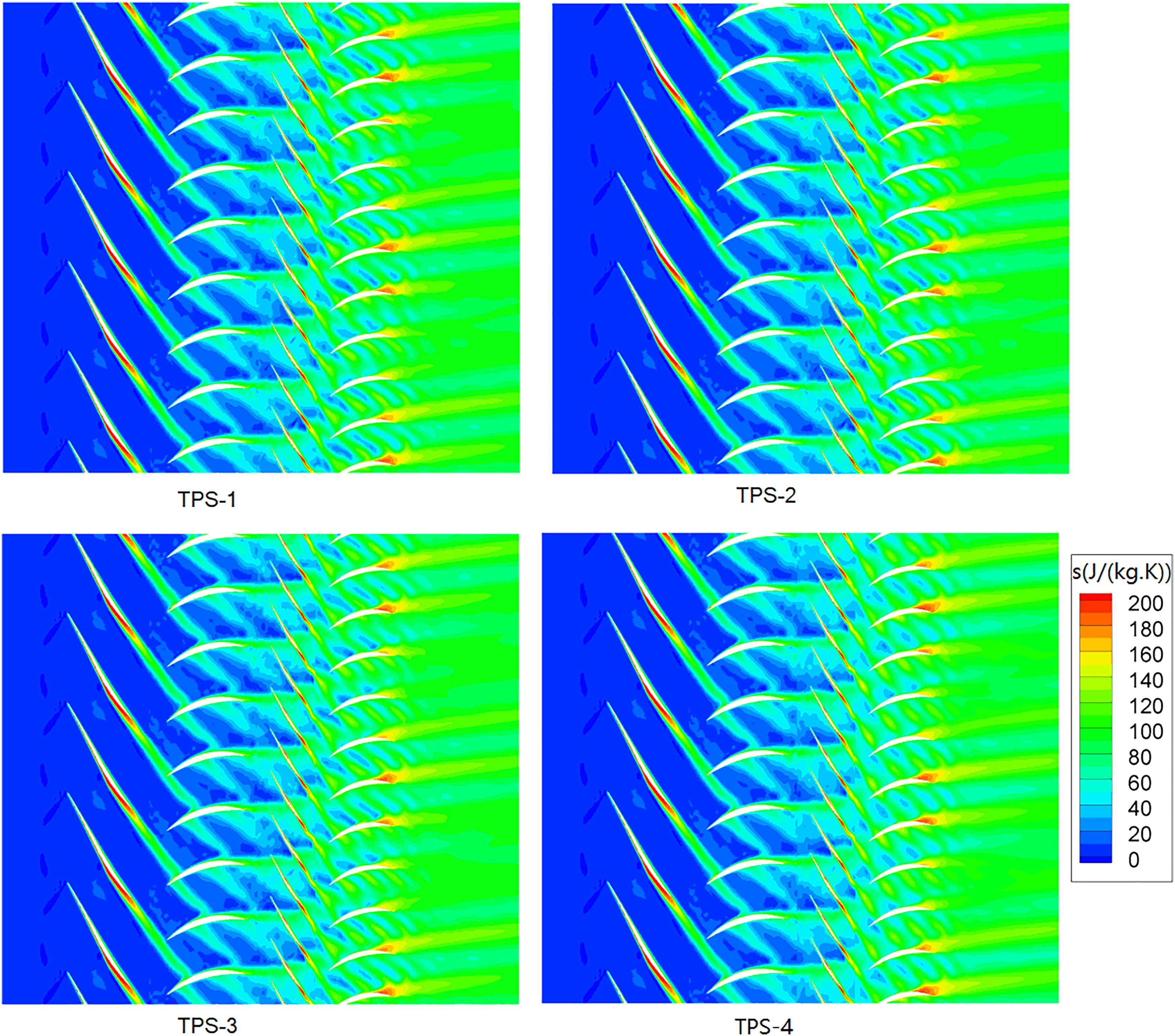
Figure 6 presents the reconstructed instantaneous entropy at 90% blade span from the four coupled time and passage spectral analyses. First, the difference in entropy contours between four analyses is not obvious, though careful examination can reveal that difference between TPS-1 and TPS-4 is the biggest and the major difference lies in the domains of row 3 and row 4. Second, at the interface between row 2 and row 3 and that between row 3 and row 4, the continuity of entropy contours of all four analyses is improved, in contrast to that of the HB-1 analysis (see Figure 3). Nevertheless, with the exclusion of more harmonics from TPS-2 to TPS-4, the entropy field continuity at the two interfaces is adversely affected.

Figure 6.

Reconstructed instantaneous entropy at 90% blade span for four coupled time and passage spectral analyses.

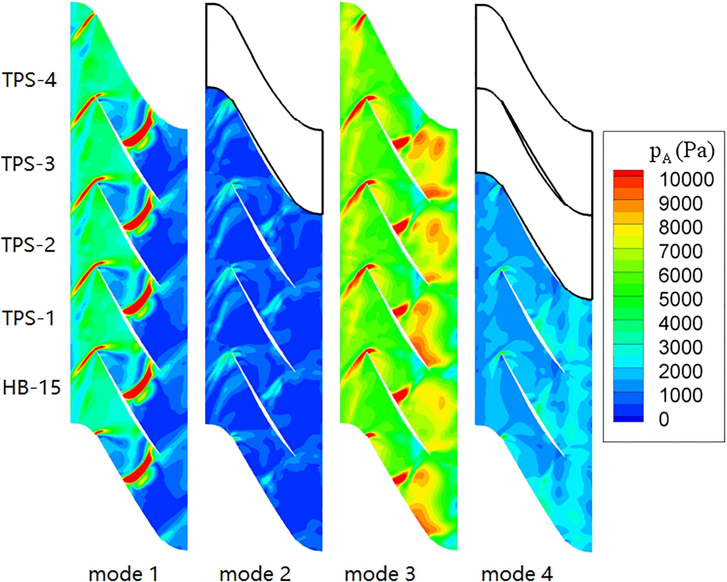
Static pressure amplitude contours of the four extra modes retained in the domain of row 3 are presented in Figure 7. In general, the results from a coupled time and passage spectral analysis are in good agreement with those from the reference HB-15 analysis. Apart from TPS-2, there is marked difference in the pressure amplitudes between other three coupled spectral analyses and the HB-15 analysis. The difference is attributed to the reflectiveness of the interface treatment which is non-reflective for plane waves only (one dimensional non-reflective). With mode 5 being resolved in the domain of row 4, the reflectiveness at the interface between row 3 and row 4 is reduced. Therefore, the results of TPS-1, TPS-3 and TPS-4 are expected to be more accurate than those of the TPS-2 and HB-15 analyses.

Figure 7.

Static pressure amplitude contours of four extra modes of row 3 at 90% span for four coupled time and passage spectral analyses and the HB-15 analysis.

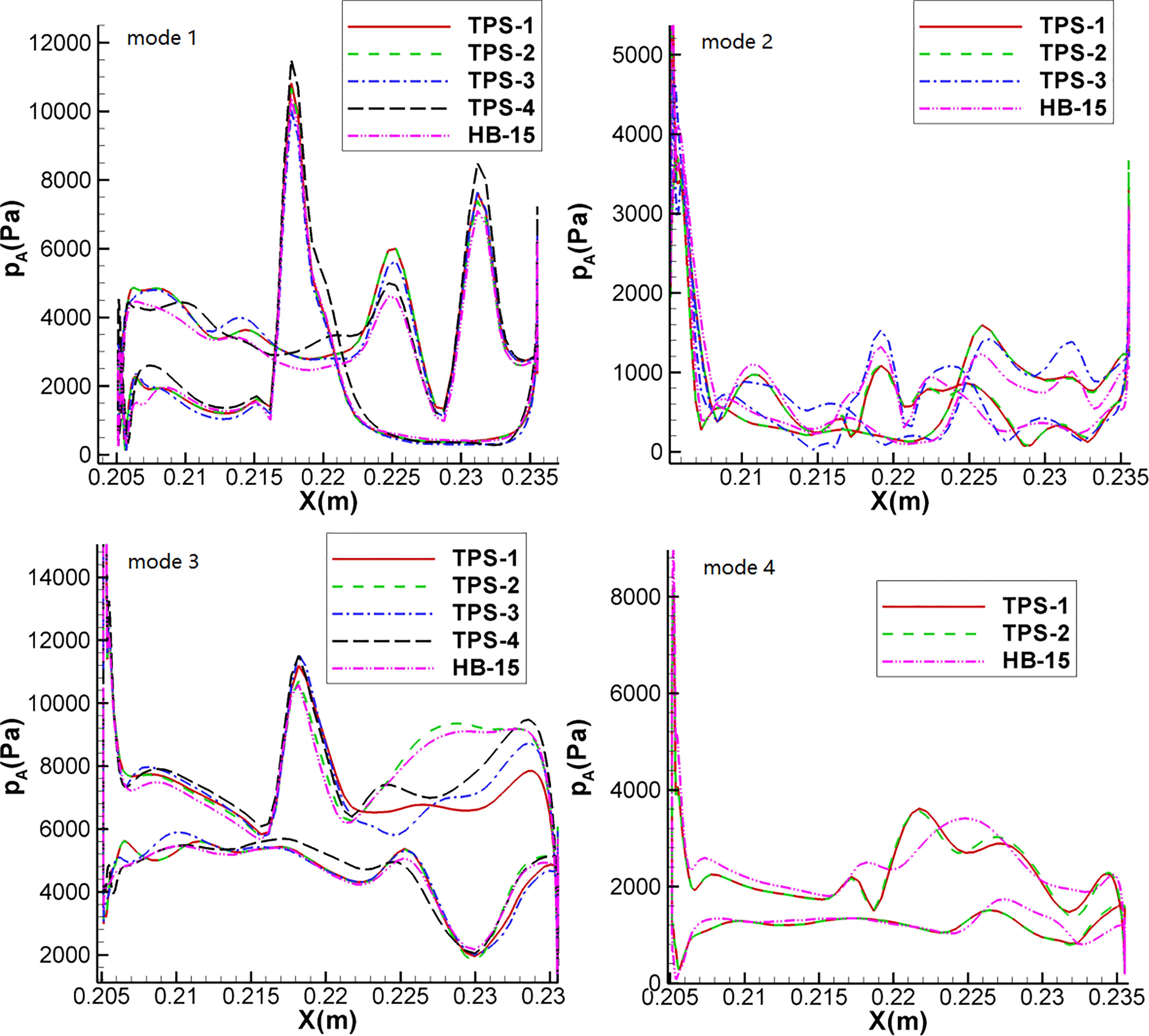
A more quantitative comparison of static pressure amplitudes on blade surface is presented in Figure 8. Same as the contours presented in Figure 7, different sets of results are generally in good agreement. Mode 1 has the best agreement among all results. Mode 3 has the biggest difference bewteeen TPS-1, TPS-3, TPS-4 and HB-15 analyses on the blade suction side around the trailing edge region. There is also marked difference between the three coupled time and passage analysis results of TPS-1, TPS-3 and TPS-4 around that region. The good agreement between TPS-2 and HB-15 is attributed to mode 5 being excluded in the domain of row 4 for the two analyses, thus both have comparable influence of numerical reflection on the solution. It can be concluded from this figure that mode 1 and mode 3 are the dominant modes and it suffices to include the two modes only in an analysis if they are of interest. Also, there is a need to employ two-dimensional non-reflective treatment at a rotor-stator interface to reduce numerical reflection.

Figure 8.

Static pressure amplitude distribution of four extra modes on row 3 blade surface at 90% span for four coupled time and passage spectral analyses and the HB-15 analysis.

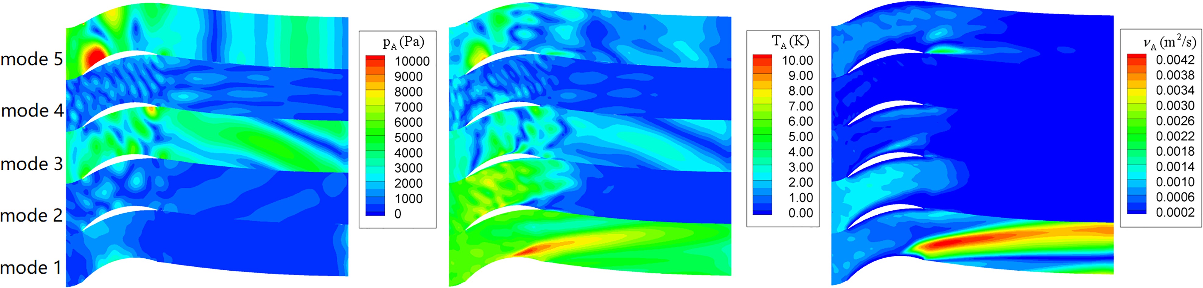
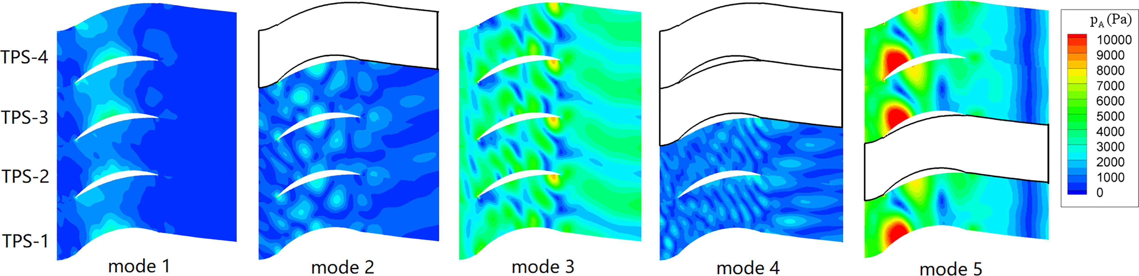
Now we examine the flow field of row 4. The amplitudes of static pressure, static temperature and turbulence quantity at 90% span are presented in Figure 9. The static pressure reveals that the dominant mode among the first four modes is mode 3, which is consistent with the four modes of row 3. Different from row 3, mode 1 is much weaker than mode 3 for row 4, which can be attributed to the weaker wakes of the second row, as shown in Figure 6 or Figure 3. It is quite interesting to see that mode 5, which is related to the wakes of row 1, is also significant. The far-reaching of row 1 wakes implies that there is a need to take this into consideration for turbomachinery aeroelastic design. The static temperature field reveals that the dominant mode is mode 1, and the second dominant mode is mode 2 and mode 3 is the third dominant mode. The picture of turbulence quantity of row 4 presents that mode 1 has the biggest content at the blade suction surface around the blade trailing edge. This is also seen from the static temperature field and the significant passage variation of instantaneous entropy field in Figure 6. Without resolving mode 1 in the domain of row 4, this significant passage variation of entropy is not captured as shown in Figure 3.

Figure 9.

Amplitudes of static pressure, static temperature and turbulence quantity of the five modes of row 4 at 90% span from the TPS-1 analysis.

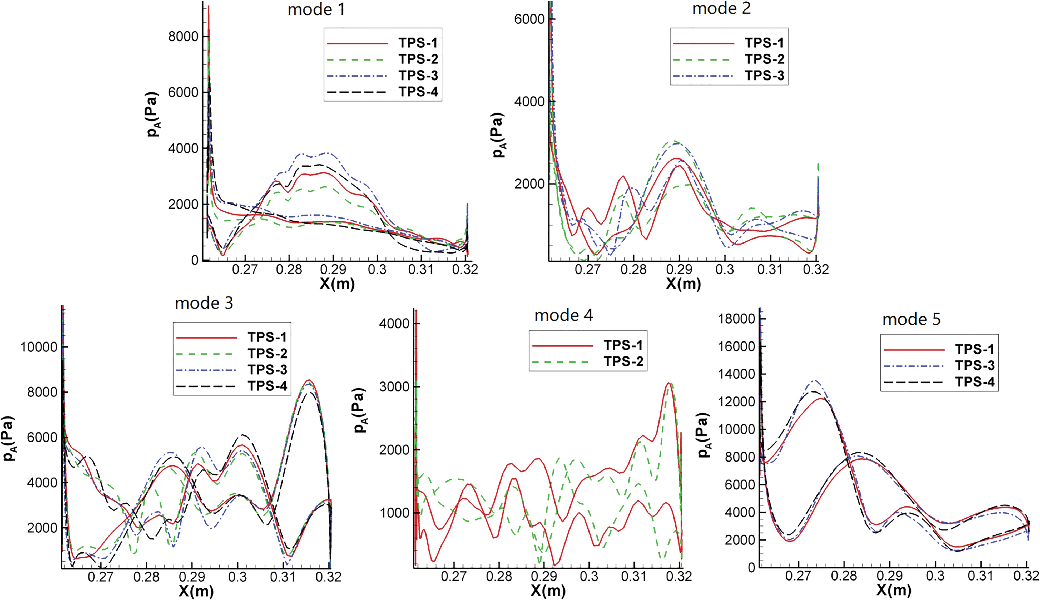
The comparison of static pressure amplitudes of the five modes for row 4 between the four different coupled time and passage spectral analyses is presented in Figures 10 and 11. For the two dominant modes: mode 3 and mode 5, the static pressure amplitudes of different analyses agree well with each other. For other three modes, the static pressure amplitudes differ significantly, particularly for mode 2 and mode 4. Further investigation is needed to find the cause of the solution variation. Nevertheless, it can be concluded that it suffices to include mode 1, mode 3 and mode 5 in an analysis to achieve desired solution accuracy.

Figure 10.

Static pressure amplitude contours of five extra modes of row 4 at 90% span for four coupled time and passage spectral analyses.

Figure 11.

Static pressure amplitude distribution of five extra modes on row 4 blade surface at 90% span for four coupled time and passage spectral analyses.

Conclusion

Two harmonic balance analyses and four coupled time and passage spectral analyses were performed to establish a priori rules for guiding the selection of time and passage harmonics for an efficient coupled time and passage spectral analysis of flow field within multi-stage turbomachines. The harmonic balance analysis using one blade passage for each blade row demonstrates the deficiency of the harmonic balance method in capturing wakes from non-adjacent upstream blade rows. With the use of multiple blade passages for a blade row, the harmonic balance method can capture wakes from non-adjacent upstream blade rows, but at much larger computational cost, which can be even prohibitive. The harmonic balance analysis using multiple blade passages reveals that the number of significant modes related to a non-adjacent upstream blade row is sparse. Four different coupled time and passage spectral analyses demonstrate that different levels of solution accuracy can be achieved by including different number of time and passage harmonics. To resolve the wakes of the second upstream blade row with acceptable accuracy, there is a need to include at least two modes: one passage harmonic and one time harmonic. The passage harmonic has zero frequency and an IBPA corresponding to the blade count of the second upstream blade row. The time harmonic has a frequency equal to the blade passing frequency of the first upstream blade row and an IBPA corresponding to the difference in blade counts of the first and second upstream blade rows. To further increase solution accuracy, one can consider including one more time harmonic, which has the frequency of the first upstream blade passing frequency and an IBPA corresponding to the summation of blade counts of the first and second upstream blade rows. Solution accuracy can be further improved by including the time harmonic with the frequency of two times the first upstream blade passing frequency and an IBPA corresponding to two times the difference in blade counts of the first and second upstream blade rows. For configuration with more than three blade rows, there is a need for the fourth and further downstream blade rows if any to resolve wakes from the third upstream blade row. One time harmonic is sufficient to capture the wakes of the third upstream blade row. This time harmonic has a frequency which is the blade passing frequency of the third upstream blade row and an IBPA corresponding to the difference in blade counts of the second and third upstream blade rows.