Introduction

Roughness usually increases the turbulent production and thus the momentum transport on aerodynamic surfaces. For an engine system, the higher momentum transport results in lower power output and poorer efficiency. For the quantitative prediction of the flow over real surfaces, various roughness properties such as the anisotropy and the magnitude of the deviation from the ideal shape must be taken into account. The equivalent sand grain roughness ks, introduced by Nikuradse (1933), establishes a relationship between surface geometry and its influence on the flow. According to this model, each isotropic roughness can be represented by a surface consisting of spheres in the densest possible arrangement, which exerts a similar influence on the flow. With the help of pipe flow experiments, Moody (1944) developed the Moody diagram, which describes an empirical relationship between the coefficient of friction λ, the Reynolds number Re, and the quotient d/Rz of pipe diameter and maximum roughness height Rz. Later, Kundu et al. (1990) defined surfaces as hydrodynamically smooth if the average height of the roughness elements is less than the thickness of the viscous sublayer (Ra<δv); i.e. a surface is hydrodynamically rough if Ra>δv. Schlichting and Gersten (2006) used the equivalent sand grain roughness and designated the flow influence of surfaces with ks⁺ < 5 as negligible. However, Schultz and Flack (2007) showed that surfaces with ks⁺ < 5 also cause a shift in the velocity profile. Sigal and Danberg (1990) introduced the shape and density parameterΛS, which takes into account the density parameter developed by Simpson (1973) and the shape parameter developed by Dirling (1973). With this parameter, the authors developed an improved prediction for evenly shaped roughness elements distributed in a regular pattern. Picking up on this work, Van Rij et al. (2002) and Bons (2005) established new correlations for the determination of extended equivalent sand grain roughness magnitudes to advance predictions for real surfaces. Using the empirical measurement results from Shockling et al. (2006), Schultz and Flack (2007) and Hohenstein (2014) developed a roughness function that predicts the shift of the velocity profile as a function of the extended equivalent sand grain roughness for ks⁺ < 20. For predominantly isotropic surfaces, the flow influence can be modeled using this extended sand grain roughness. Loss effects of strongly anisotropic roughness, such as an increase in turbulent dissipation rate, do not follow the predictions (Kurth et al., 2018).

Real surfaces which are worn in operation generally consist of anisotropic and isotropic structures (Gilge et al., 2019), which is why a surface parameter that can quantify the loss effects for such surfaces is crucial. To increase the understanding of the interactions between anisotropic and isotropic roughness elements, channel flows over rough surfaces with anisotropic and isotropic roughness components are simulated by means of DNS. To evaluate the interactions between the roughness structures, anisotropic and isotropic roughness components are first simulated separately and then superimposed. The directional dependence of the anisotropic components is taken into account by changing the angle of attack (AoA). The AoA is the relative angle between the flow direction and the preferred orientation of anisotropic roughness and corresponds to xs+ in Table 3. The simulations are carried out with a constant friction Reynolds number

resulting in a constant force driving the flow. Thus, flow losses are observed in the mass flow and turbulent quantities, such as dissipation and production.

Governing equations

Incompressible and isothermal channel flows of Newtonian fluids are studied, and therefore the general Navier-Stokes equations are simplified to form the governing equations:

A block-structured, finite-volume solver with Immersed Boundary Method (IBM) implemented in foam-extend-4.0 for channel flows is used to solve the equations. Second-order accuracy both in time and space is achieved with Gauss linear spatial and backward temporal discretization. With the help of DNS, small-scale turbulent fluctuations are resolved in time and space without having to resort to turbulence models. In contrast to empirical measurements, calculated flow variables are available over a wide area and in the direct vicinity of the wall, so that comprehensive analyses are possible. For rough surfaces, the necessary surface-conforming mesh is associated with a disproportionately high computational effort, which is why the IBM is applied instead. The IBM approach enables simulations on Cartesian grids by dividing the grid into solid cells and fluid cells. Cell centers of solid cells are located within the overflown body and the velocities in these cells are set to zero. For the chosen IBM approach, the velocities in fluid cells which share a face with a solid cell are obtained via quadratic interpolation between the wall and neighboring fluid cells. A more detailed explanation and validation of the IBM can be found in Senturk et al. (2016). Sampling errors of time averaged velocities are calculated as in (Ries et al., 2018) and specified with error intervals in the respective figures.

Examined surfaces

The separability of the aerodynamic effects of the roughness structures is achieved, by first simulating anisotropic and isotropic roughness components separately, and then superimposed. A total of seven channel flows, over surfaces with isotropic and anisotropic roughness structures, are simulated with different flow directions, as shown in Table 1. The doubly infinite channel consists of two identical rough surfaces (Figure 1). The lengths are reported in non-dimensional form and valid for all channels considered in this work. Non-dimensional quantities

Figure 1.

Doubly infinite channel (isotropic surfaces).

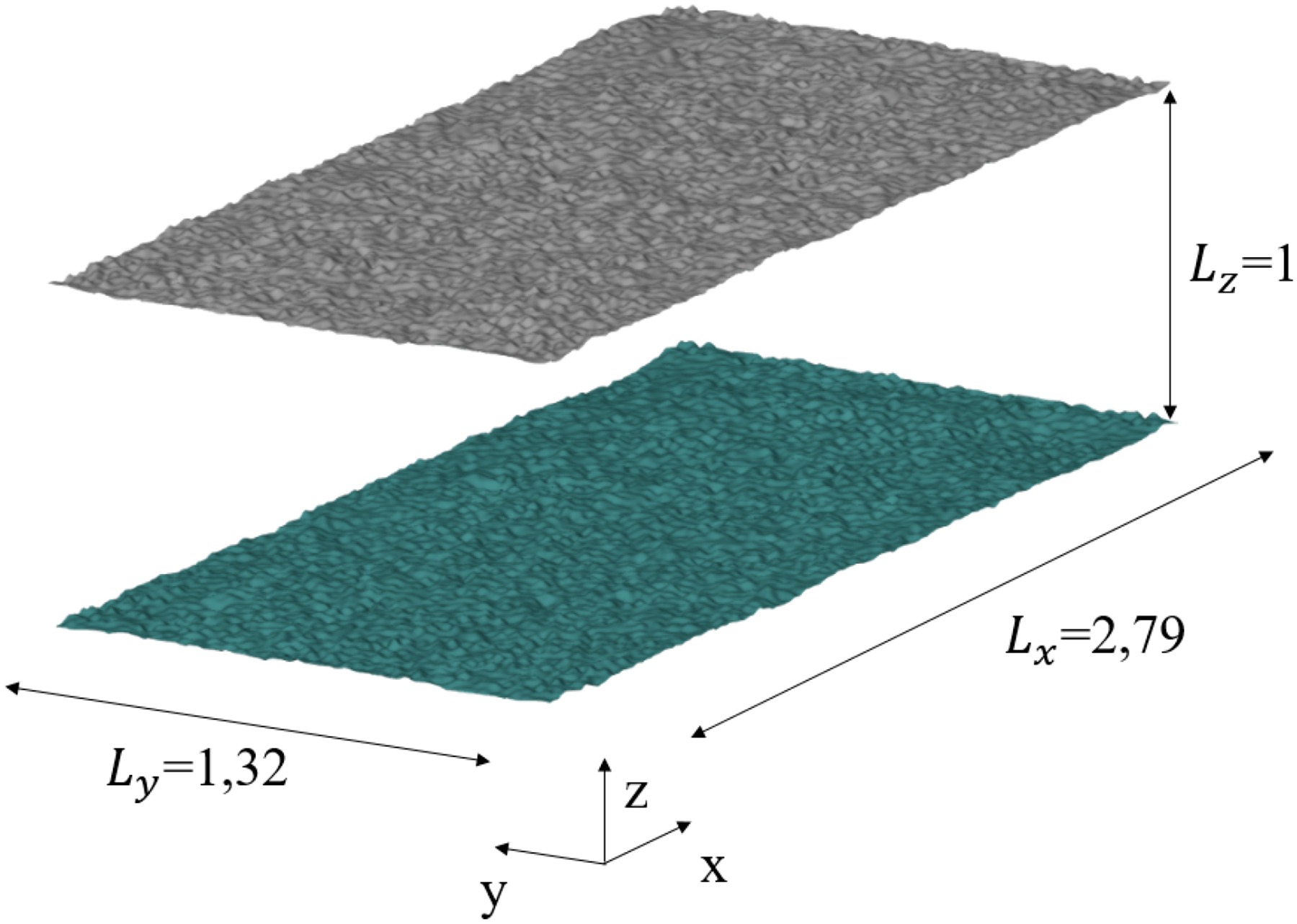
For the isotropic surface, a real surface, worn in operation with an isotropy coefficient of Str=0.75 (DIN EN ISO, 25178-2:2012), is chosen. For better separability of the effects, no real surface is chosen for the anisotropy, but a synthetically created one. The height values of the synthetic roughness follow a sinusoidal function with period s+=252.5 and amplitude of z+=6. Such dimensions for anisotropic roughness elements could for example be found on worn compressor blades as in Gilge et al. (2019).

Besides the separate examination of the effects on the flow, the interactions are considered through the superposition of the surfaces. Superposition is accomplished by adding the height values of the surfaces, i.e. the coordinates in the z-direction. Since perfectly isotropic surfaces do not occur in reality, the flow influence of the selected isotropic surface is not fully independent of the AoA. The dependence is suppressed by rotating the isotropy with the AoA before superposition. The flow passes the isotropic structures with the same AoA, while the AoA changes for the anisotropic structures. The centered evaluation area is aligned with the flow direction to compare identical isotropic structures. In Table 3, the evaluation areas (gray) and corresponding z+-diagrams are visualized. To generate the z+-diagrams, a cut (red) is placed through the center of the evaluation area. The diagrams demonstrate that the rotation of isotropy before superposition leads to identical isotropic roughness elements for each cut. The given maximum roughness heights Sz are the average of sectional Sz values when uniformly dividing each surface into 25 segments. The equivalent sand grain roughness is calculated as in Bons (2005) using Sz as roughness height kh.

Table 3.

Roughness parameters, top view of evaluation areas (gray box) and z+ diagrams.

Roughness	Sz+	ks+	Evaluation area	z+-diagram
Isotropic	13.84	10.35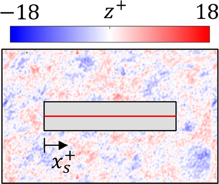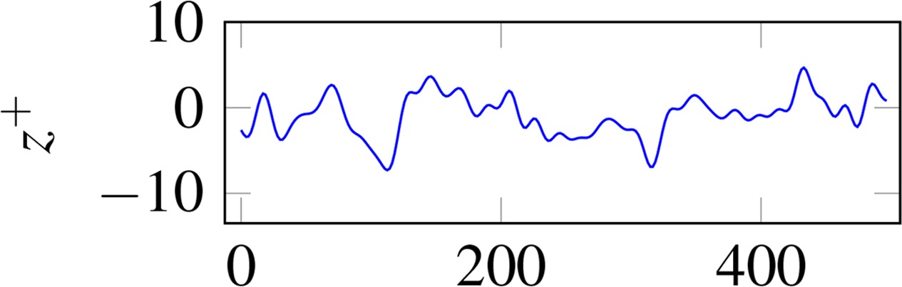
Anisotropic 90∘	12	4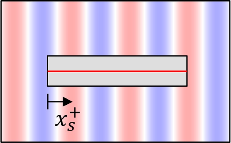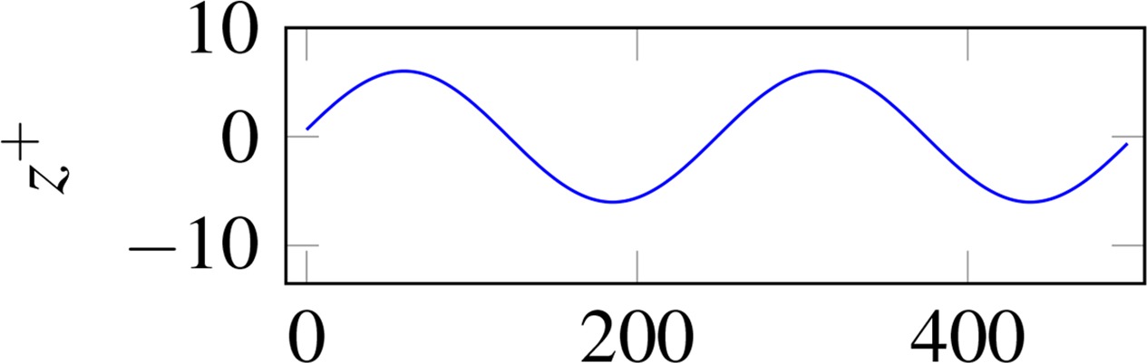.23
Superimposed 90∘	21.29	16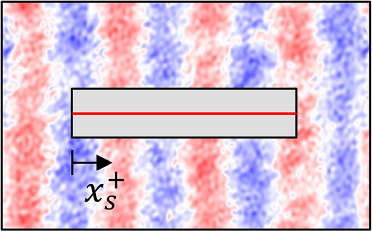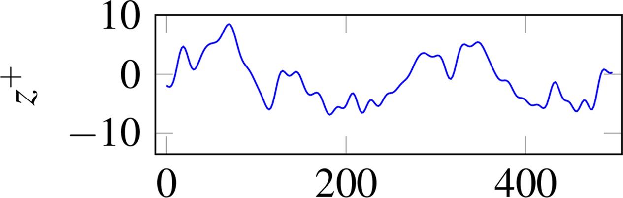.87
Anisotropic 60∘	12	3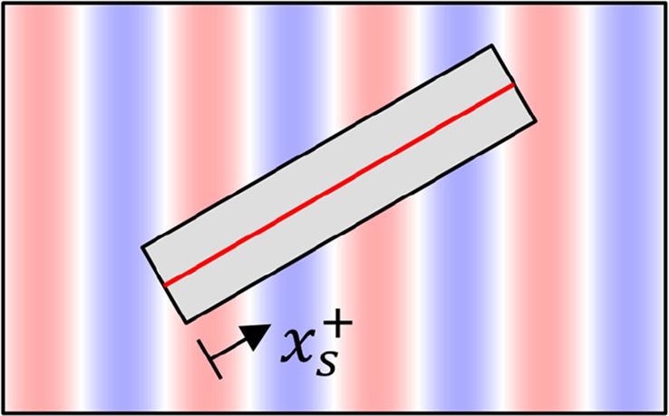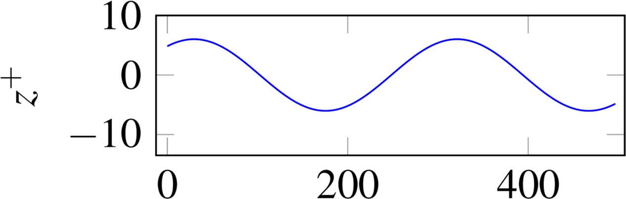.61
Superimposed 60∘	22.2	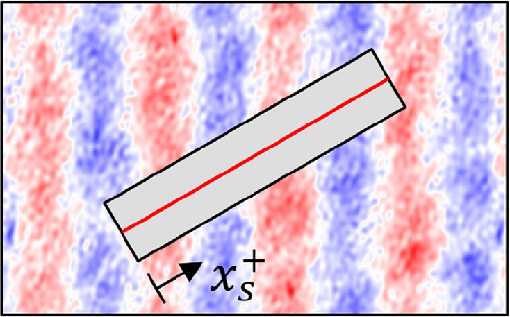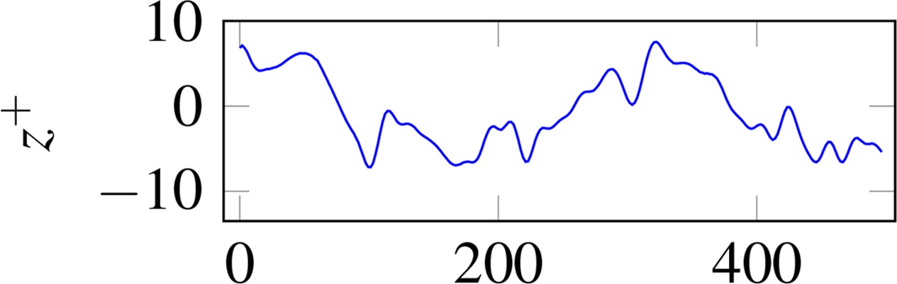16
Anisotropic 30∘	12	1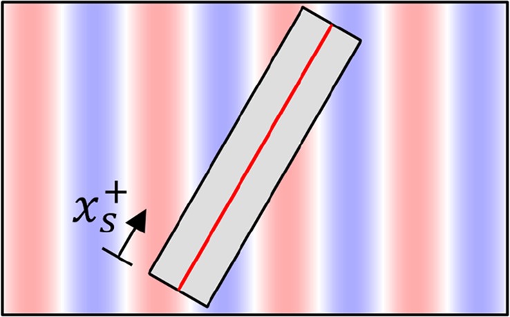.91
Superimposed 30∘	21.22	13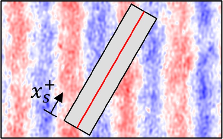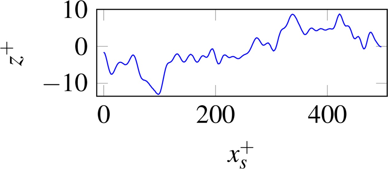.99

The mesh parameters for the doubly infinite channel are listed in Table 4, with Δz+ and Δzc+ as the cell heights at the wall and the channel center, respectively. The IBM was validated by Kurth et al. (2021) for smooth and rough surfaces with DNS simulations from Moser (1999) and Thakkar et al. (2017), respectively. The mesh study demonstrates that the chosen mesh resolution is sufficient for the applied roughness resolution of Δx+=Δy+=1.8. Roughness resolution is the non-dimensional distance in x and y between two data points of the rough surface. The time step is set so that the Courant-Friedrich-Lewy stability condition with CFL < 1 as given by Courant et al. (1928) is satisfied for each time step. First, the simulations are run until the initial transients are complete and the flow is fully developed. The non-dimensional simulation duration of this step is t⁺ = 50. Time-averaged quantities are obtained with an additional simulation duration of 80 < t⁺ < 100, which is sufficient for statistical convergence according to Thakkar (2017).

Results and discussion

The profiles of non-dimensional and time-averaged resulting velocities

plotted against z+ are shown in Figure 2. For each AoA a line in the z-direction from the bottom surface to channel half-height is sampled. The velocity profile for a channel with smooth walls from Moser (1999) is shown for reference.

Figure 2.

Non-dimensional velocity profiles for AoA (a) 90°, (b) 60°, and (c) 30°. The sampling error is 0.6% for AoA = 90° and less than 0.075 for the remaining simulations. The results for the smooth case are from Moser (1999).

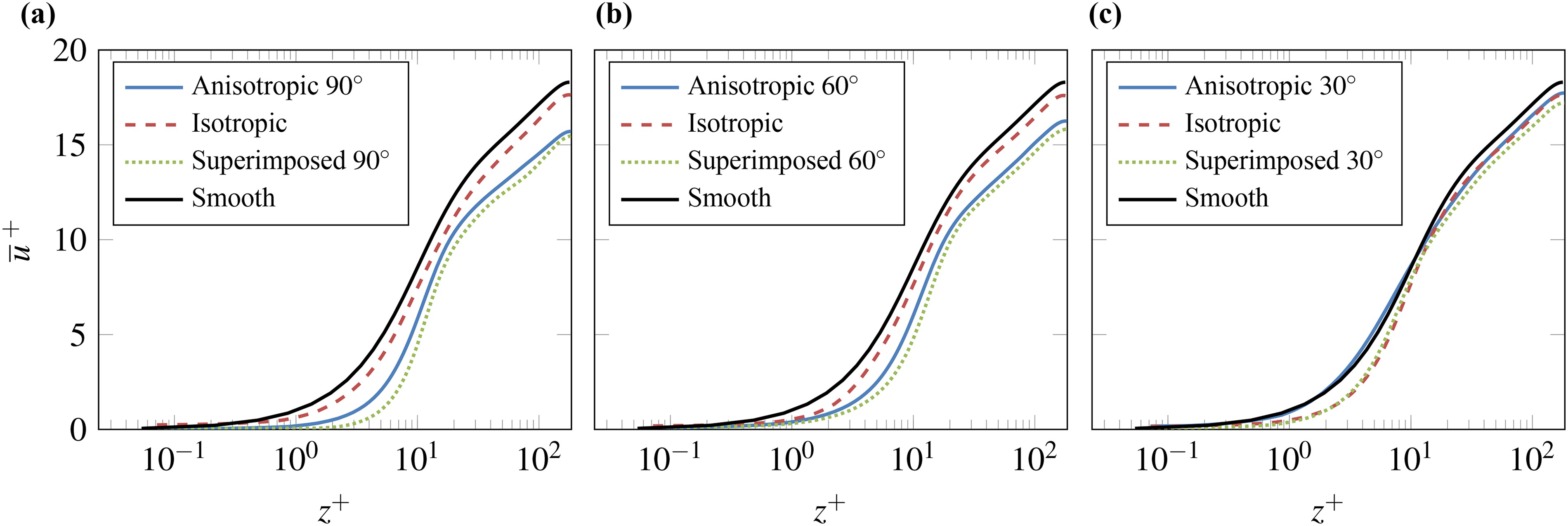
The highest velocities occur for the smooth surface. The profiles of the isotropic, anisotropic, and superimposed surfaces are shifted downwards. As the AoA decreases, the shift for anisotropic and superimposed profiles becomes less pronounced. According to Thakkar (2017), the parallel, downward shift of the velocity profiles to the channel flow with smooth walls is a measure of an increase in the surface friction of the flow. However, the applied constant friction Reynolds number corresponds to a constant drag force for the calculated simulations. Hence, the bulk Reynolds numbers

integrated over the evaluation areas are compared as a measure for the mass flows. In Figure 3 the results are shown with the percentage deviation of the Reynolds number to the case with smooth walls above the bars.

Figure 3.

Mean Reynolds numbers in the evaluation areas with percentage deviations from the smooth channel. The sampling error is 0.6% for AoA = 90∘ and less than 0.075% for the remaining simulations. The results for the smooth case are from Moser (1999).

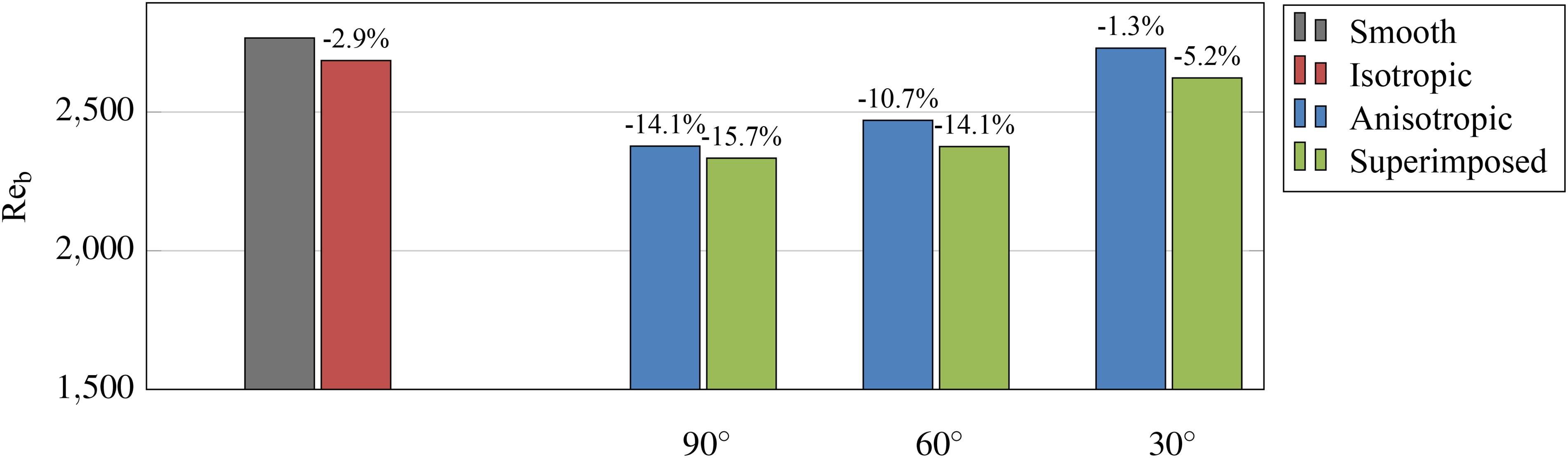
Consistent with the shifts in the velocity profiles, a non-linear relationship between reduction in mass flow and the AoA is observed for anisotropic and superimposed surfaces. The surfaces were positioned such that the volume of the channels remains constant for all cases. Hence, the reduction of the effective cross-sectional area due to anisotropic roughness peaks reaches a maximum for AoA = 90°, and decreases as the AoA decreases. The reduction in mass flow correspondingly decreases, so that Re_b of the anisotropic surfaces approaches that of the smooth surface. When comparing the additional reduction in mass flow due to isotropic roughness elements for the superimposed surfaces for each AoA, it is evident that the anisotropic structures mitigate the isotropic effects for high AoAs and amplify them for low AoAs. Thus, the reduction in mass flow is driven predominantly by the anisotropic elements for high AoAs, and by the isotropic elements for low AoAs. The observed reduction in mass flow for anisotropic and superimposed surfaces contrasts with the calculated roughness parameters in Table 3. The largely non-linear function of the AoA does not follow the changes in ks⁺ values.

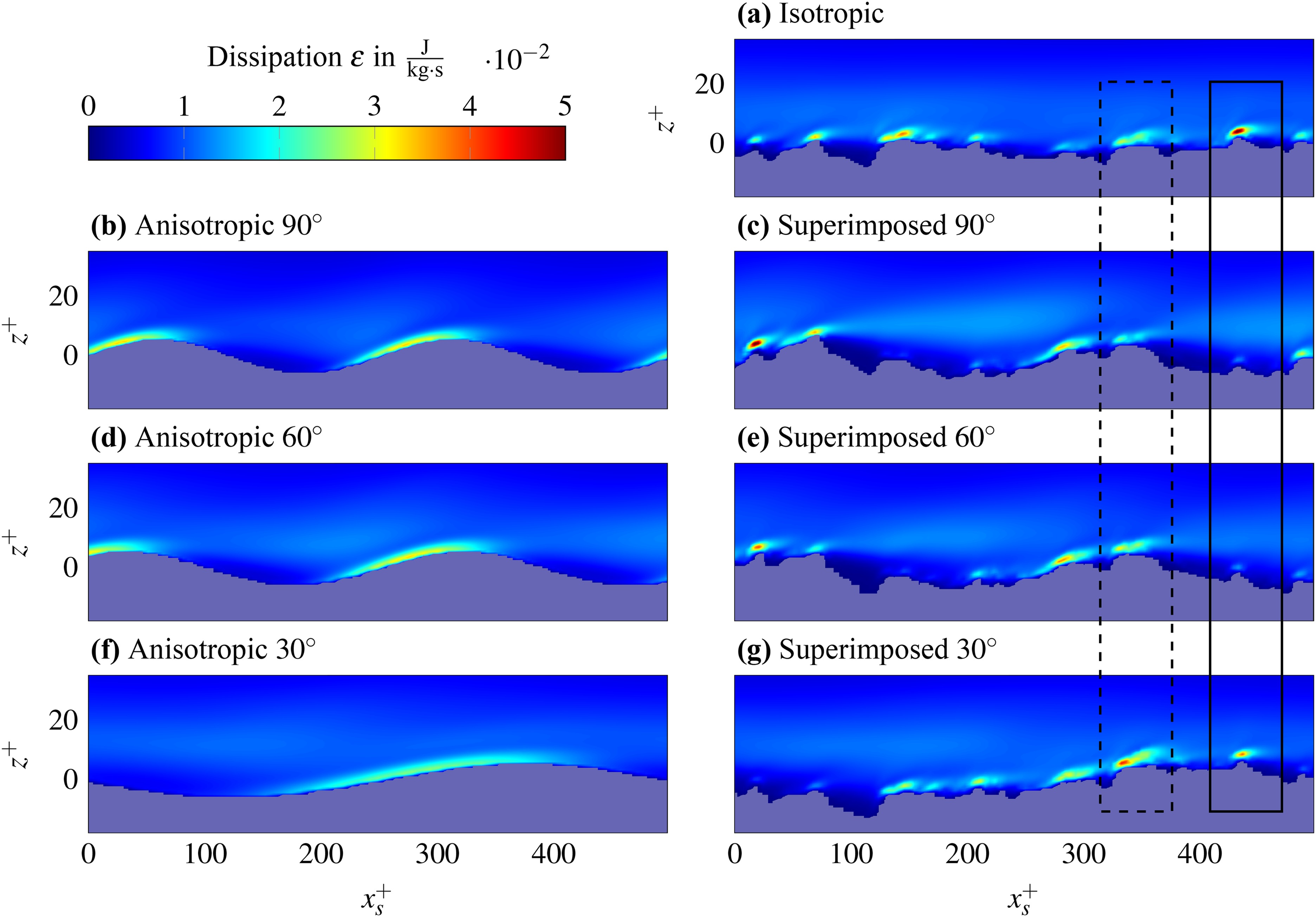
For further investigation of the interactions, turbulent production

and dissipation rate

are studied as the main features for turbulent losses and are shown in Figures 4 and 5. The flow domain is sectioned according to Table 3.

Figure 4.

Turbulent production (surface in purple).

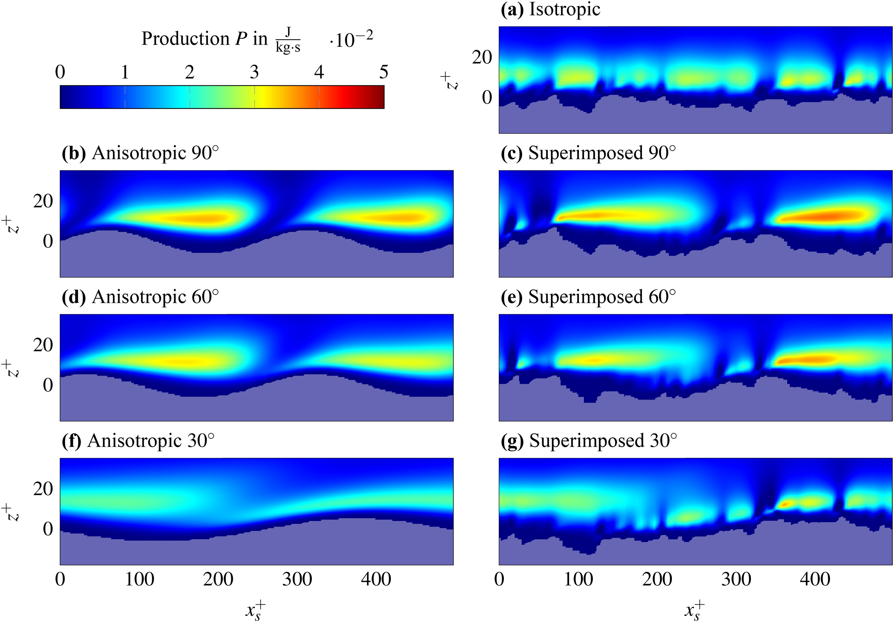
Within the viscous sublayer and roughness valleys, the turbulent production reduces to a minimum. Similarly, the turbulent dissipation rate tends towards a minimum in roughness valleys, and reaches a maximum on rising flanks and roughness peaks. The flow is accelerated on rising flanks of the anisotropy by a local negative pressure gradient. Accordingly, the flow is decelerated by descending flanks, driven by a local positive pressure gradient. The black box in Figure 5 shows that combination of isotropic roughness elements with a negative pressure gradient leads to a local reduction of the dissipation rate. Conversely, the dashed box shows that the dissipation rate is increased when superimposed with a positive pressure gradient. Regions of increased production form cone shapes for the anisotropic surfaces. For the superimposed surfaces the shapes are punctuated by the isotropic elements. The cone geometries become less pronounced with decreasing AoA and converge towards the shapes of the isotropic surface. This observation agrees with the analysis of the reduction in mass flow, to the extent that for high AoAs the losses are driven by the anisotropic elements, and by the isotropic elements for low AoAs.

Figure 5.

Turbulent dissipation rate (surface in purple).

The effects can only be assessed locally with these figures. To investigate the global, turbulence intensity is considered. According to Roach (1987), flows with domain-averaged turbulent kinetic energy

different from zero are at a turbulence level, which is defined by the turbulence intensity:

Normalization of turbulent kinetic energy with the time-averaged velocity provides a comparison of the turbulent levels at different mass flows. In Figure 6 the turbulence intensities are shown, calculated with the turbulent kinetic energy and velocities integrated over the channel volume.

Figure 6.

Turbulence intensity integrated over channel volume. The sampling error is less than 0.005 percentage points for all simulations.

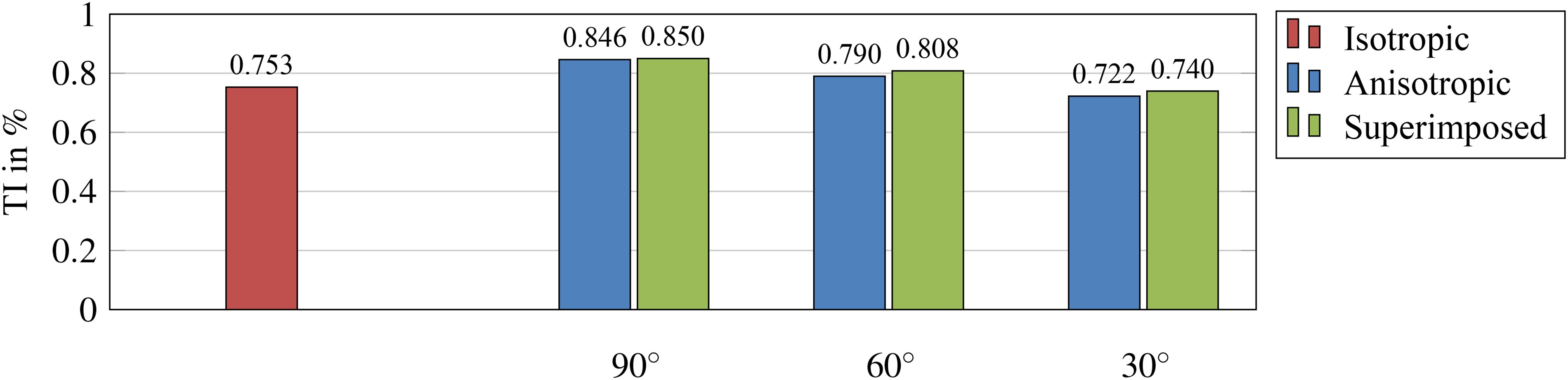
The bar chart suggests that the state of the turbulent boundary layer depends on the AoA. The turbulence intensity is strongly dependent on the anisotropic roughness structures, and increased only to a small extent when the isotropic roughness is superposed. The turbulence level reaches a maximum for AoA = 90° and decreases slightly with decreasing AoA.

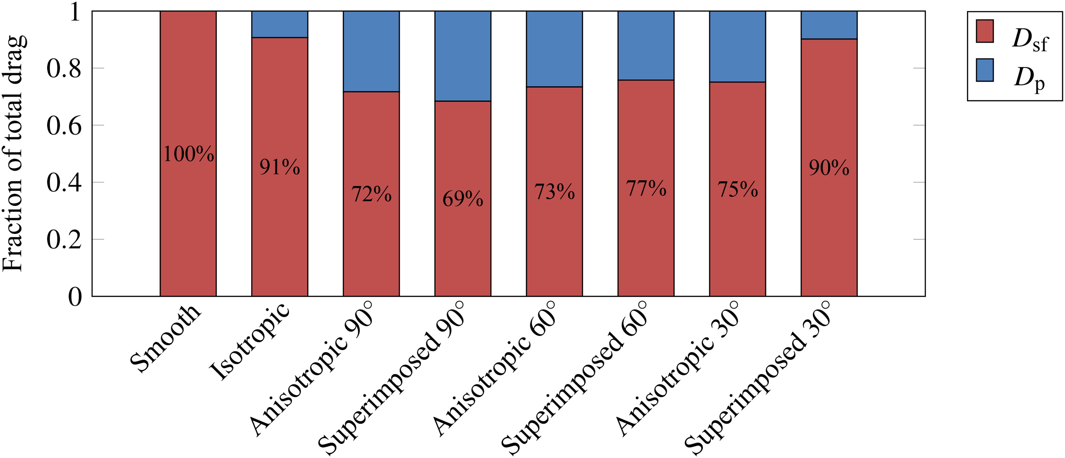
As a final step, the effects of the roughness structures on the drag are analyzed. The total drag in the direction of the flow is composed of forces tangential to the wall (skin friction drag) and normal to the wall (pressure drag). For a constant friction Reynolds number Reτ = 180 and channel dimensions as in Figure 1, a total drag force

acts in all channels, with A being the surface area. The ratios of pressure drag and skin friction drag are evaluated and are shown in Figure 7. The proportion of the skin friction drag is given as a percentage. For the smooth surface, the total drag is composed exclusively of frictional forces. Accordingly, the pressure drag for anisotropic and superimposed surfaces decreases with decreasing AoA. Isotropic roughness structures increase or decrease the pressure drag depending on the AoA. The pressure drag is primarily dependent on the profile shape of the surface, which explains the drop in relative pressure drag with decreasing AoA. The similar values for AoA = 90° and the increase in skin friction drag for the superimposed surface with AoA = 30° agrees with the observation that for high AoAs the flow behavior is determined by the anisotropic components and for low AoAs by the isotropic components.

Figure 7.

Ratio of skin friction drag and pressure drag. The given percentage values belong to the skin friction drag. The results for the smooth case are from Moser (1999).

Conclusions

Economical preservation of the functionality of overflowed surfaces requires the prediction of roughness-induced loss effects on the flow. An increased understanding of the interactions between anisotropic and isotropic roughness elements has been achieved through DNS of channel flows over real surfaces. The investigations performed in this work demonstrate that, in order to predict flow losses of anisotropic and superimposed roughness structures, roughness functions solely dependent on the equivalent sand grain roughness are not suitable. It was shown that the flow losses are strongly dependent on the orientation of the anisotropic structures.

For surfaces with superimposed roughness structures, the reduction in mass flow becomes maximum for an AoA = 90° and decreases in a non-linear relationship to the AoA. A comparison with the losses of the isotropic and anisotropic surfaces showed that the maximum loss is primarily determined by the anisotropic roughness structures. The additional reduction in mass flow due to isotropic elements is mitigated by the anisotropic elements for high AoAs and amplified for low AoAs. Thus, as the AoA decreases, the influence of anisotropy decreases, and the loss behavior is increasingly driven by the isotropy. Consideration of turbulent production and dissipation rate has shown that the turbulent losses are largely determined by the pressure gradients of the anisotropic structures. A locally positive pressure gradient corresponds to a rising flank, and a negative gradient to a descending flank. Thereby, a local maximum is generated by the superposition of an isotropic roughness element with a positive pressure gradient, and a local minimum by the superposition with a negative pressure gradient. An evaluation of the turbulence intensity showed that the boundary layer flows are at a higher turbulent level for increasing AoAs. The turbulence intensity decreases analogously to the mass flow in a non-linear relationship to the AoA. Finally, it was found that the composition of the total drag for superimposed surfaces changes as a function of the AoA.

To improve the prediction of reduction in mass flow for superimposed surfaces, a new correlation of the simulation results with the calculated ks⁺ values is conceivable. It was shown that for high AoAs the loss effects are predominantly driven by the anisotropy and for low AoAs by the isotropy. Consequently, existing surface parameters, which determine the preferred direction of anisotropy, can be used for the AoA-dependent roughness function developed in this way. Future investigations should therefore pursue a detailed analysis of the turbulent behavior of the boundary layers for different AoAs and variations of anisotropy and isotropy.

Nomenclature