Baseline configuration

The experiments were performed in a subsonic cascade wind tunnel at the LMFA, Lyon, whose characteristics are precisely detailed by (Dawkins et al., 2021). This cascade is set in order to precisely control the inlet flow, which consists in the inlet endwall boundary layer, the inlet angle and the inlet turbulence. The cascade parameters are presented in Table 1. Bleeding channels are used to remove the boundary layer developing on the endwall 0.5 stator chord (c) upstream of the channels. For each flow condition, the bleeding flow is altered to retrieve the same pressure profile around the endwall leading edge. This set up ensures a thin and repeatable inlet boundary layer for all inflow conditions. This enables to observe a classical, repeatable corner separation behaviour downstream of the cascade. 25 pressure tapings are used to best fit the pressure distribution along the profile at midspan against a database of numerical flow predictions obtained at angle increments of 0.1. This enables to measure the inflow incidence with a precision of ± 0.05⁰ for the investigated blade. The inlet turbulence is generated by a grid 280 bar widths upstream of the cascade and measured 0.25c upstream of the leading edge of the blades.

The performance of the cascade is measured with a five-hole probe (Pt) in a plane at 0.2c downstream of the trailing edge, along with inlet pitot tubes (Ps,∞,Pt,∞) for inflow pressures reference. Their respective positions are shown in Figure 1. The total pressure losses are computed as

Figure 1.

Side view of the rig.

The integrated pressure losses ωT are defined as the mass-averaged pressure losses on the whole plane of measurement. The profile losses ωMID are defined as the mass-averaged pressure losses at the same axial position, but at midspan only. The endwall pressure losses are defined as the difference between the integrated pressure losses and the profile losses:

This baseline configuration is intended to be used as an open test case for corner separation studies, and was precisely designed and characterised by (Dawkins et al., 2021) for that purpose. The high aspect ratio of the blade is made on purpose to uncouple the midspan flow from the near-endwall flow and to isolate the corner separations occurring at the two roots of the blade. The midspan profile trailing edge separation starts at the incidence i = 5.5°, and develops further upstream as the incidence is increased. Moreover, endwall losses rapidly increase with the incidence, from approximately 0.9% at i = 0° to 4.3% at i = 5.4°, and are obtained with an experimental uncertainty of ±0.1%. This is shown later in the Results and Discussion section. As such, this precisely controlled cascade exhibits an important corner separation, and can therefore be used for evaluating a control device such as guide fins.

Guide fin manufacturing and insertion

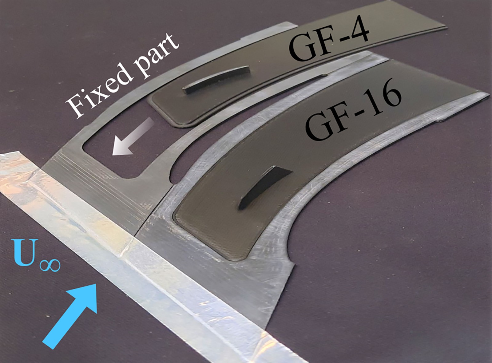
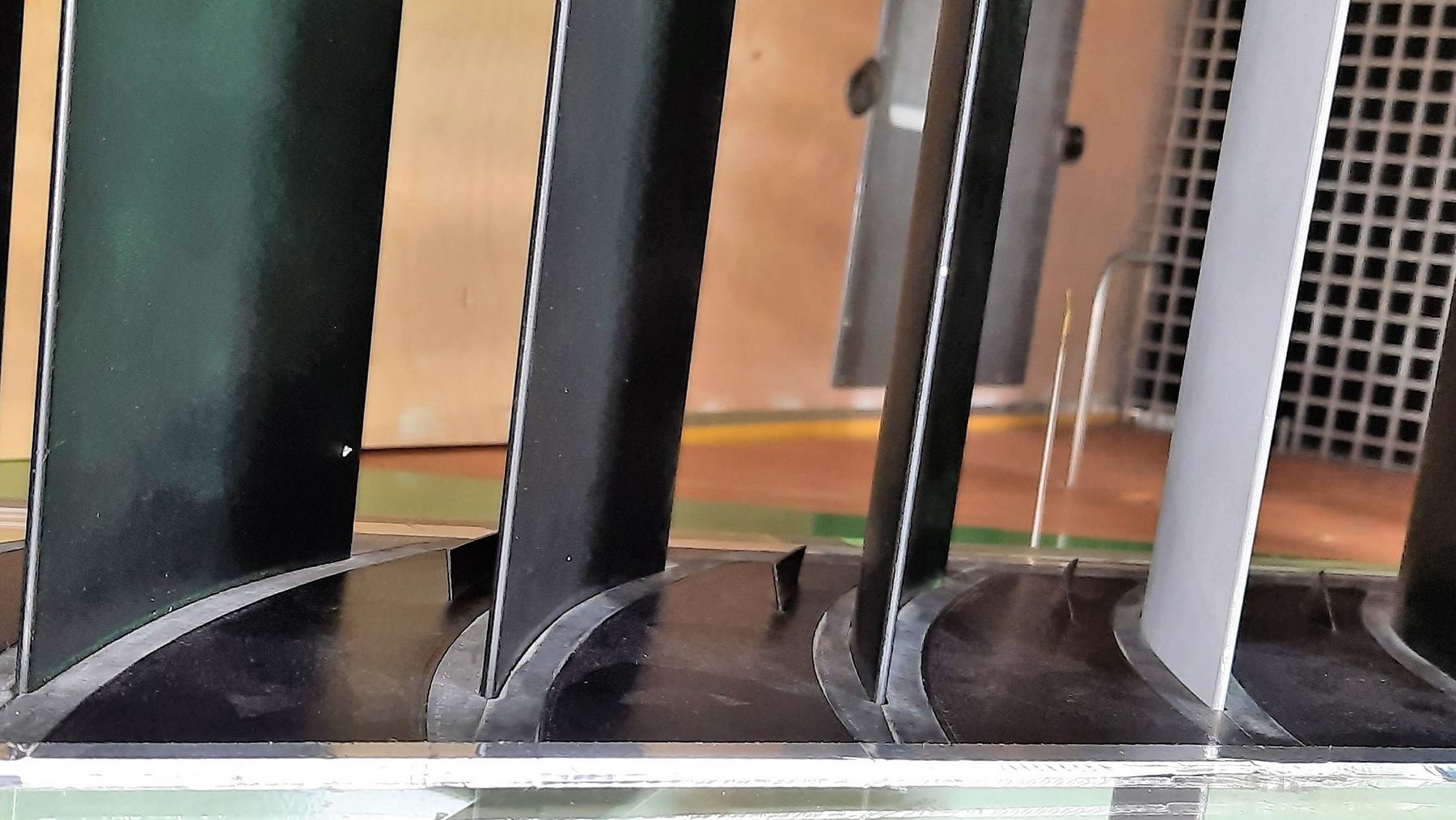
An insertion system was designed to equip six neighbouring channels with guide fins, on both endwalls. It is made of a fixed part fitting the stator profile in which a removable part containing the guide fin can be slid in. Figure 2 illustrates this principle, and Figure 3 its implementation in the cascade. The system is 2 mm thick, yielding a section reduction of about 1.3%. Its upstream part starts at an axial position 0.29c upstream of the stator leading edge. It consists of a ramp that smoothly brings the flow up, from the endwall to the top of the platform, with an angle seen by the flow of 3.8°. This system, including the guide fin, is manufactured with a Fuse Deposition Modelling (FDM) method, using ABS plastic. A nozzle of 0.4 mm diameter is used, as well as a precision of 0.09 mm per layer. With this system, a complete set of 12 guide fins is manufactured in about 30 hours, which is much faster than with a conventional process. In order to limit extra losses and the inlet boundary layer thickening, the fixed part is sanded down to a rugosity of 0.5 µm. The same operating points are reached with and without the insertion system. Nonetheless, adding this system necessarily alter the reference flow. A flat platform was then slid in the insertion system to mimic the initial baseline configuration. This modified baseline is characterised experimentally by the authors, and is the one used in this paper. This way, the gain measured when replacing the flat platform by a platform with a guide fin is independent of the insertion system. Moreover, a variation of the endwall losses below the experimental uncertainty is found at several incidences when comparing the initial and modified baseline. This yields a negligible effect of the system.

Figure 2.

Illustration of the insertion system, with GF-4 and GF-16. U∞ refers to the upstream velocity.

Figure 3.

Rear view of the system in the cascade.

This experimental set up thus enables to assess the influence of a guide fin on endwall losses. Next section describes a RANS-based methodology implemented to find manufacturable guide fins that efficiently reduce the endwall losses.

Guide fin parametrisation

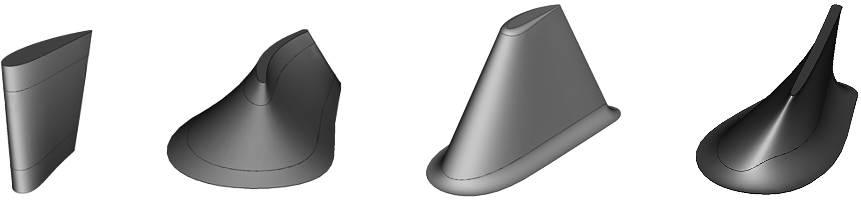
In order to ensure an aerodynamic shape, the guide fin is built using several aerofoils stacked at different spanwise locations, from hub to tip. So as to reduce the total number of parameters, it is chosen to build only one parametrised aerofoil, whose parameters values are a function of its spanwise location. The evolution of each parameter is chosen to be linear, because it requires only two values and still allows the construction of complex geometries. Finally, two fillets can be added to round the junctions between the hub and the sides, and between the tip and the sides. Examples of guide fins generated with the following methodology are shown in Figure 4.

Figure 4.

Examples of guide fins of various shape complexity.

Aerofoil parametrisation

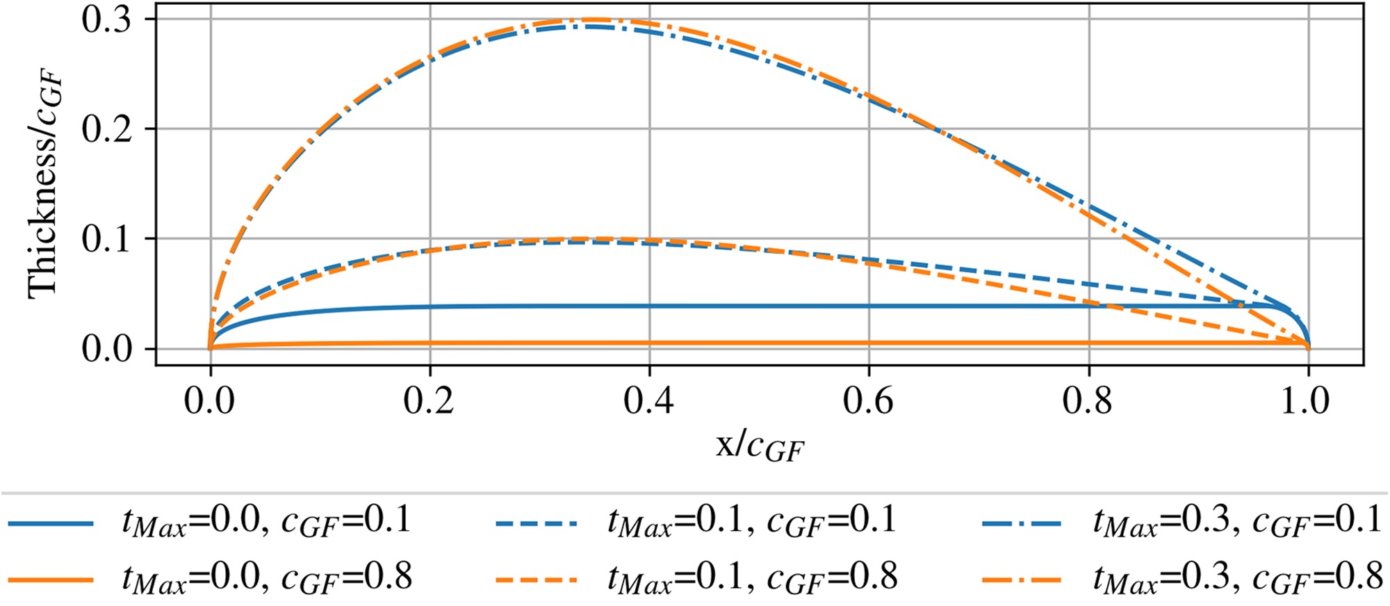
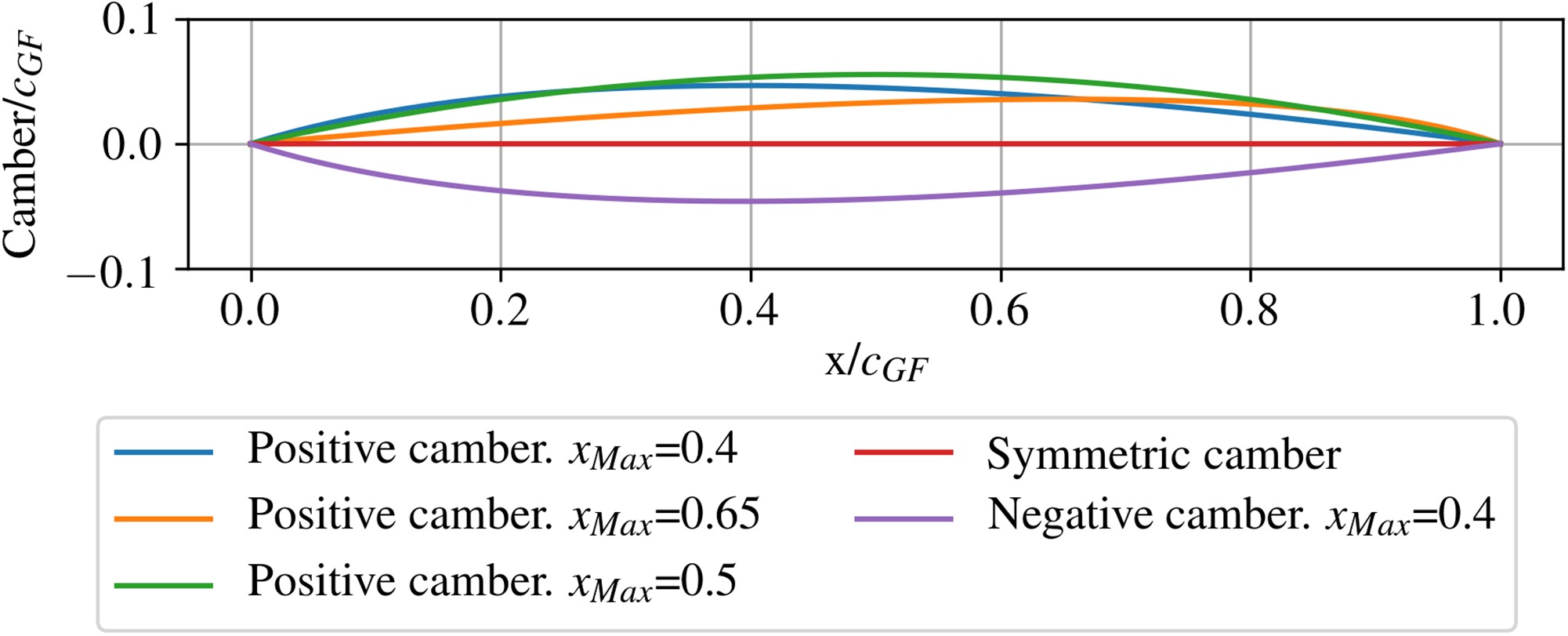
The parametrised aerofoil is built from a parametrised thickness law and a parametrised camber law. A thickness law of reference is built with the BEZIER-Parsec 3333 parametrisation described in (Salunke et al., 2014), in which geometrical parameters can be easily set and tuned. In order to stay close to the simplest thickness laws, no inflexion points are permitted. From then, the parametrised thickness law is obtained by tuning the maximum thickness value. A circular trailing edge (TE) is added so that the dimensioned aerofoil has a constant trailing edge thickness, fixed to the smallest manufacturable value shown in Table 2. Examples of thickness laws are shown in Figure 5. The camber law is obtained from a spline of order 2 constrained by three parameters: the position of the maximum of camber and the values of its tangents at the edges. Several examples are shown in Figure 6. Providing a chord value and a two-dimensional position is then sufficient to define an aerofoil with 7 parameters. Given a linear evolution, a hub aerofoil, a tip aerofoil and a height value define an entire guide fin with 15 parameters.

Table 2.

Manufacturing constraints.

Manufacturing constraint	Value
Absolute minimum fillet radius	5 mm
Absolute value of TE thickness	0.5 mm
Maximum sweep or lean angle at LE or TE	45°
Absolute minimum value of guide fins chord	25 mm
Absolute minimum guide fin height	1 mm

Figure 5.

Thickness laws for different guide fin chords (cGF) and maximum thicknesses (tMax).

Figure 6.

Camber laws for different maximum positions (xMax) and tangents at the edges.

Efficient design space exploration accounting for manufacturing constraints and design experience

The 17 degrees of freedom of the parametrised guide fins may lead to guide fins which are irrelevant in terms of aerodynamic expertise or do not respect manufacturing and positioning constraints (see Table 2). In order to reduce the design space to geometries of interest for the user, two new parametrisations are proposed with the following characteristics: (a) for all values of the new parameters, the associated value of the original 17 ones can be easily retrieved and (b) all geometries generated by the new parameters satisfy the manufacturing and positioning constraints. The first parametrisation involves only 4 new parameters presupposed to have a significant impact on the losses. This defines a relatively small subdomain easier to explore and mostly based on design experience. These 4 parameters correspond to the guide fin height, the inlet and outlet metal angles, and the curvilinear position on a midpitch line (see Figure 7) around a rather simple, two-dimensional aerofoil of reference. Their values is described in Table 3. The second parametrisation consists of 16 new parameters, allowing for more complex shapes. Guide fins can have very 3D geometries. Thin tip aerofoils and thin to thick hub aerofoils are considered. As tip fillet radii would be very small, no tip fillets are considered. Hub fillet radius varies between 0 and 75% of the guide fin height. Lean and sweep parameters varying between ±25° are introduced. The position of maximum camber varies in [30%cGF, 60%cGF]. Moreover, guide fins are forced to be relatively aligned with the local stator camber line. The angle between the tangent to the stator camber line and the x-axis is computed. The guide fin metal angles vary in [−5°, +5°] with respect to this angle at the corresponding axial positions, except for the inlet hub angle that varies in [−20°, +5°]. Finally, relatively short guide fins with a height in [0.8%c, 8%c] are considered, with a minimum chord of 0.2c, and the authorised positions are extended to the blue surface shown in Figure 8.

Figure 7.

All guide fins of DOE-4.

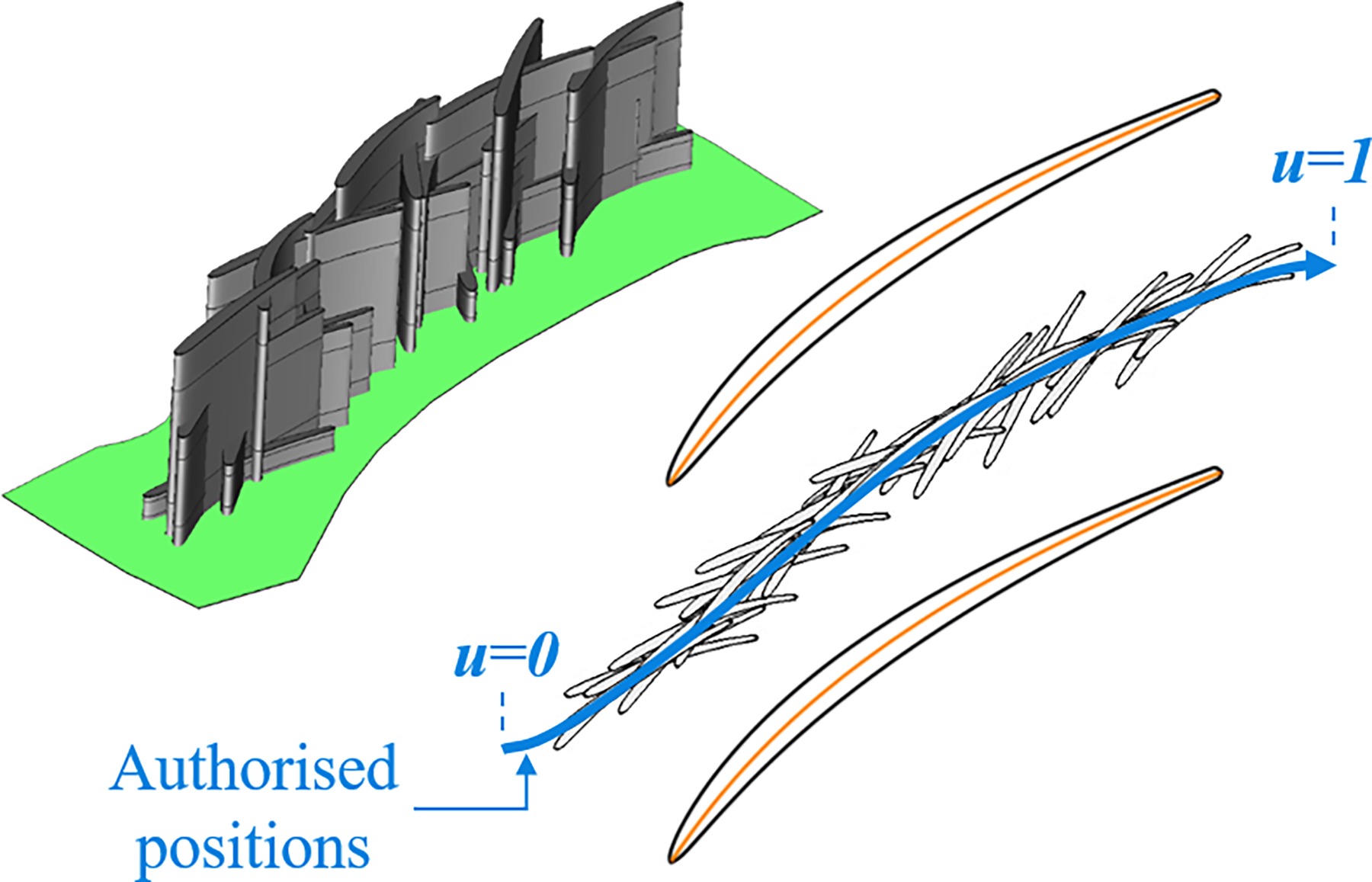
Table 3.

DOE-4 parameters range and value %c and %cGF refer to percentages of stator and guide fin chord.

Parameter		Value
Height	∈	[0.8%c, 20%c]
LE metal angle β1	∈	[20°,65°]
TE metal angle β2	∈	[0°, β1]
Position on midpitch line u	∈	[0.14,0.88]
Chord	=	30%c
Position of maximum camber	=	55%cGF
Maximum thickness	=	4.5%cGF
Radius of tip and hub fillets	=	0

Figure 8.

Several guide fins of DOE-16.

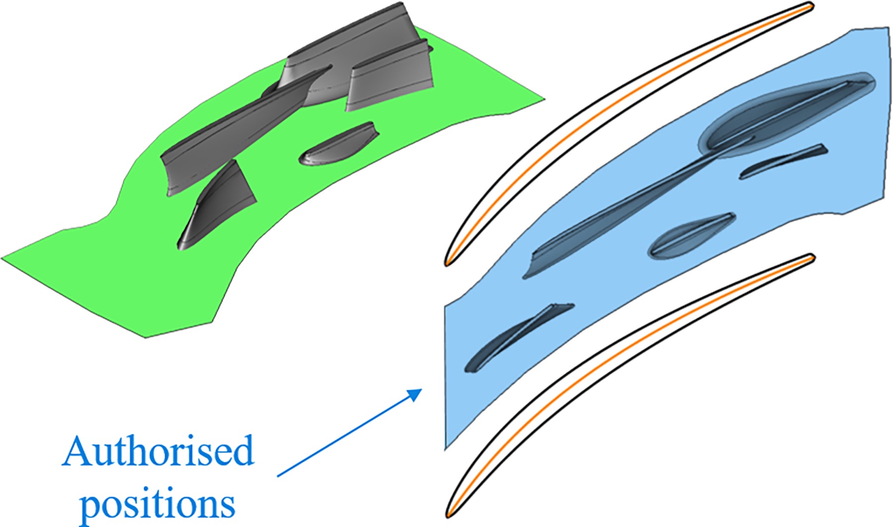
Unfortunately, even these new parametrisations cannot guarantee that any geometry generated at random in these reduced design spaces will be associated with a RANS prediction. Indeed, the surface generation, the meshing process or the computation itself could fail in case of too complex geometries. In order to generate a design of experiments (DOE) which best explores the design space of admissible guide fins (i.e. with an available RANS result), an original and specific strategy for handling such computational failures is used. First, for each parametrisation, a large database of guide fins is generated using a Monte Carlo methodology and only the guide fins with viable CAD surfaces are kept. The main assumption in the algorithm used is that such large databases are representative of the set of all admissible geometries. The DOE is then built by picking a small subset which spans as best as possible the entire database. To achieve this, the “kernel herding” algorithm proposed by (Chen et al., 2010) is used. It consists in minimising the distance between the empirical distribution defined on the DOE and the one on the entire dataset. For the first parametrisation with 4 parameters, the corresponding DOE (DOE-4) with 40 geometries is shown in Figure 7. For the second parametrisation with 16 parameters, the corresponding DOE (DOE-16) contains 160 geometries. 5 of them are shown in Figure 8. Later in the paper, RANS results associated with each DOE are presented. Respectively 100% of the DOE-4 and 80% of the DOE-16 is successfully associated with a RANS result. These high viability rates ensure that both subdomains are indeed well explored.

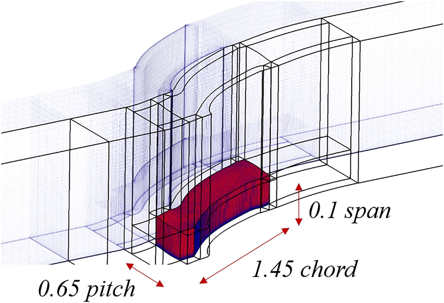
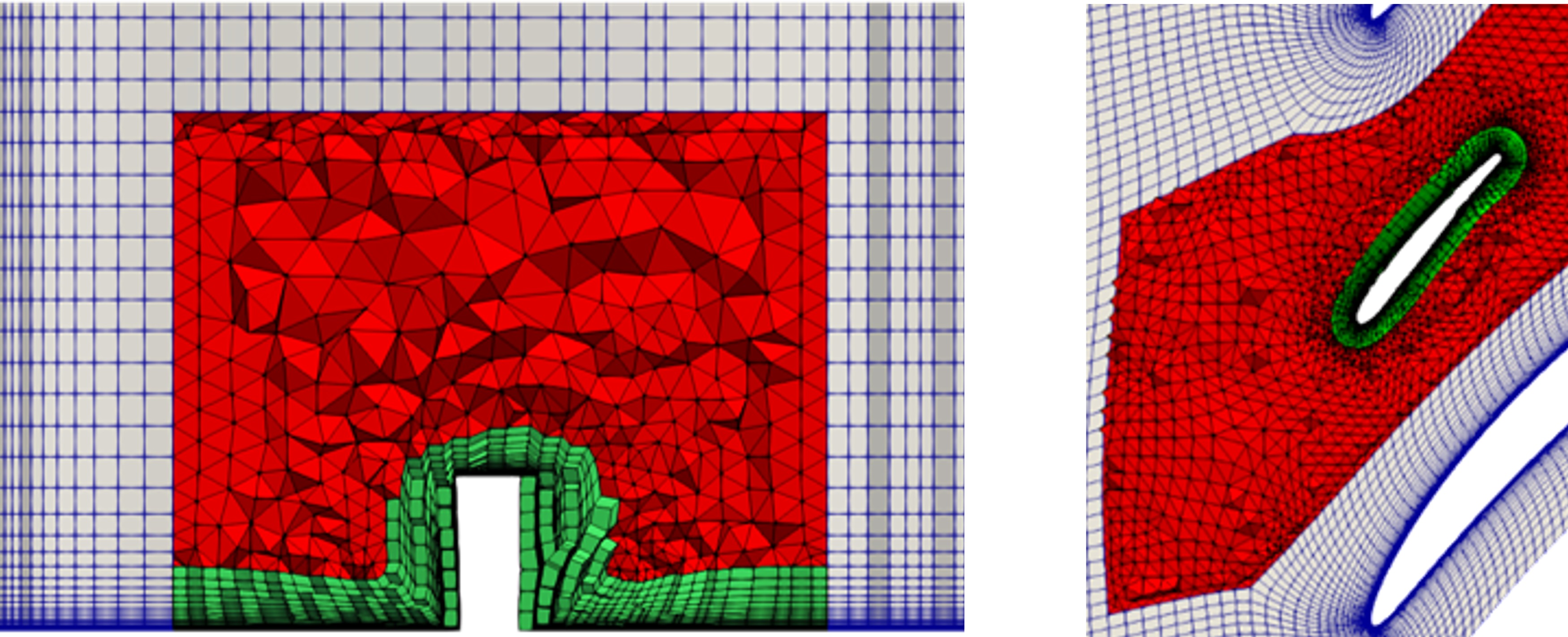
Hybrid meshing strategy

In order to save computational time and to uncouple the spatial discretisation of the two geometries, the stator part is meshed separately from the guide fin part and is fixed. Attention is paid to generate these meshes consistently with one another. A structured O-4H mesh of a single channel of the baseline cascade is obtained using AutoGridV5 (Numeca). It contains approximately 1.1×106 hexahedral cells, and is characterised by a maximum y+ value of 4 in the leading edge region. A symmetry plane is used at midspan. Blocks are then rearranged to centre the mesh on the channel, and to define one block of controlled dimensions, in red in Figure 9. The structured O-grid block is not modified to ensure a systematic, high quality discretisation of the profile boundary layer. The red block is then replaced by an unstructured mesh containing the guide fin. This results in a hybrid mesh containing both structured and unstructured blocks. The unstructured red block is generated automatically using the software ANSA (Beta). It is made of 24 prisms layers that grow from and in a direction normal to the solid surfaces, of tetrahedra and of pyramids. Efforts are made to have elements as square as possible at the interface to enhance the quality of the pyramids. Prisms and pyramids automatically connect to the red boundaries, thus ensuring grid point coincidence. The growth rate at the interface is set to 1.2 for both volumes to ensure its continuity, yielding an unstructured block of typically 3.5×105 cells with a guide fin, and 1.7×105 cells without. Figure 10 shows portions of a hybrid mesh with a guide fin and illustrate the consistence of the two meshes.

Figure 9.

Unstructured block boundaries In red. Black lines: block borders. A second faded channel is added for visualisation purposes only.

Figure 10.

Portions of hybrid mesh with a guide fin White elements: hexahedra (structured part). Green elements: prisms. Red elements: tetrahedra and pyramids.

CFD set up

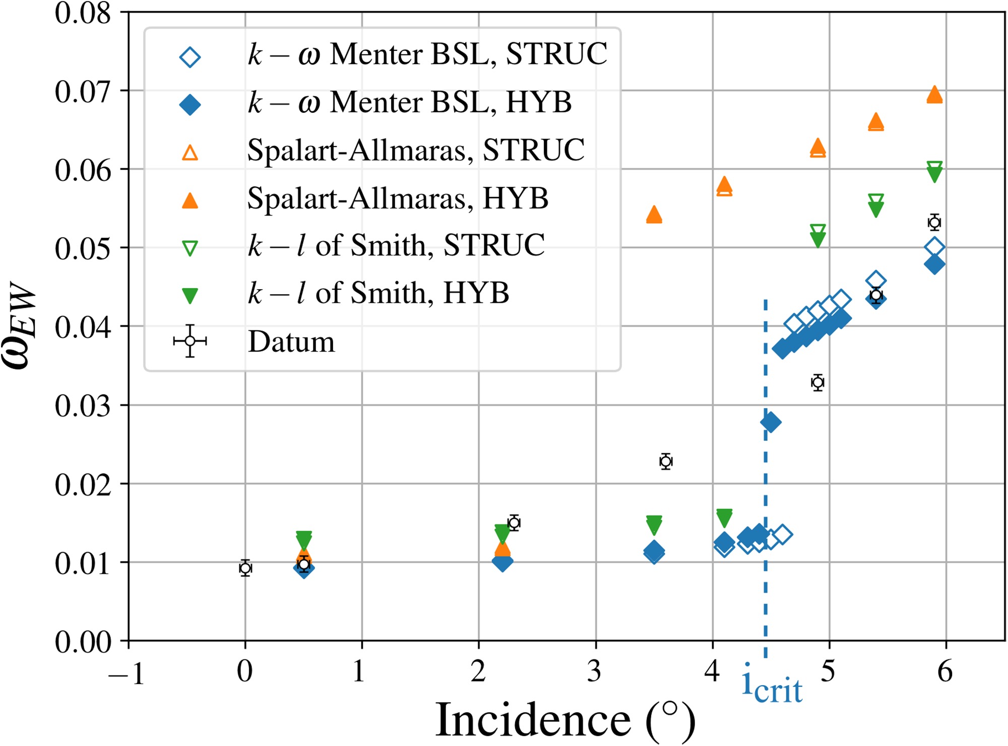
RANS results are computed using the CFD solver elsA (ONERA). In order to validate the meshing methodology, results obtained on the fully structured mesh of reference and on the hybrid mesh without guide fin are compared in Figure 11, using the turbulence models of Spalart-Allmaras, k−l of Smith and k−ω Menter BSL. The spatial scheme of Roe of order 2 is used with no limiter for variable reconstruction at interfaces. Among these three turbulence models, k−ω Menter BSL is found to best retrieve the experimental wake profiles at midspan and the downstream endwall boundary layer thickness, with both meshes. Using the hybrid mesh lowers the critical incidence by 0.2° to icrit=4.4∘. Above i = 4.6°, the endwall losses differ by about 0.2%, but the gradient with respect to the incidence is identical. Given the sensitivity to the numerical environment, these differences are not surprising and remain acceptable. The capability of the solver elsA to perform RANS computations on hybrid meshes is therefore validated. DOE-4 and DOE-16 will therefore be evaluated using hybrid meshes, with k−ω Menter BSL.

Figure 11.

Evolution of the endwall losses on the measurement plane. STRUC and HYB respectively refer to results obtained using the structured mesh of reference and the final hybrid mesh without guide fins. The same post-processing is used for both experimental and numerical data.

Results of the design of experiments

Respectively 40 and 129 viable guide fins are selected for the DOE-4 and the DOE-16. The present work focuses on guide fins that act on a large range of incidences, while not deteriorating too much the losses at the design incidence. As guide fins are designed to act on the near-endwall losses, it is not relevant to evaluate them at incidences where separation at midspan occurs. As a consequence, endwall losses are monitored at an incidence near-design, i = 0.5°, and before the midspan separation, at i = 4.9°. Results are gathered in Figures 12 and 13, together with the RANS prediction of the baseline case for comparison purposes.

Figure 12.

CFD results of DOE-4.

Figure 13.

CFD results of DOE-16.

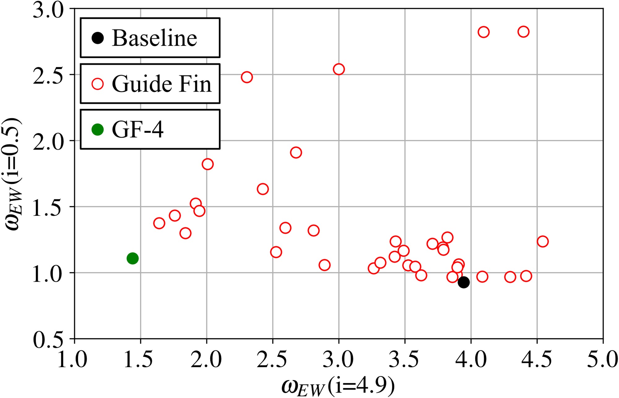
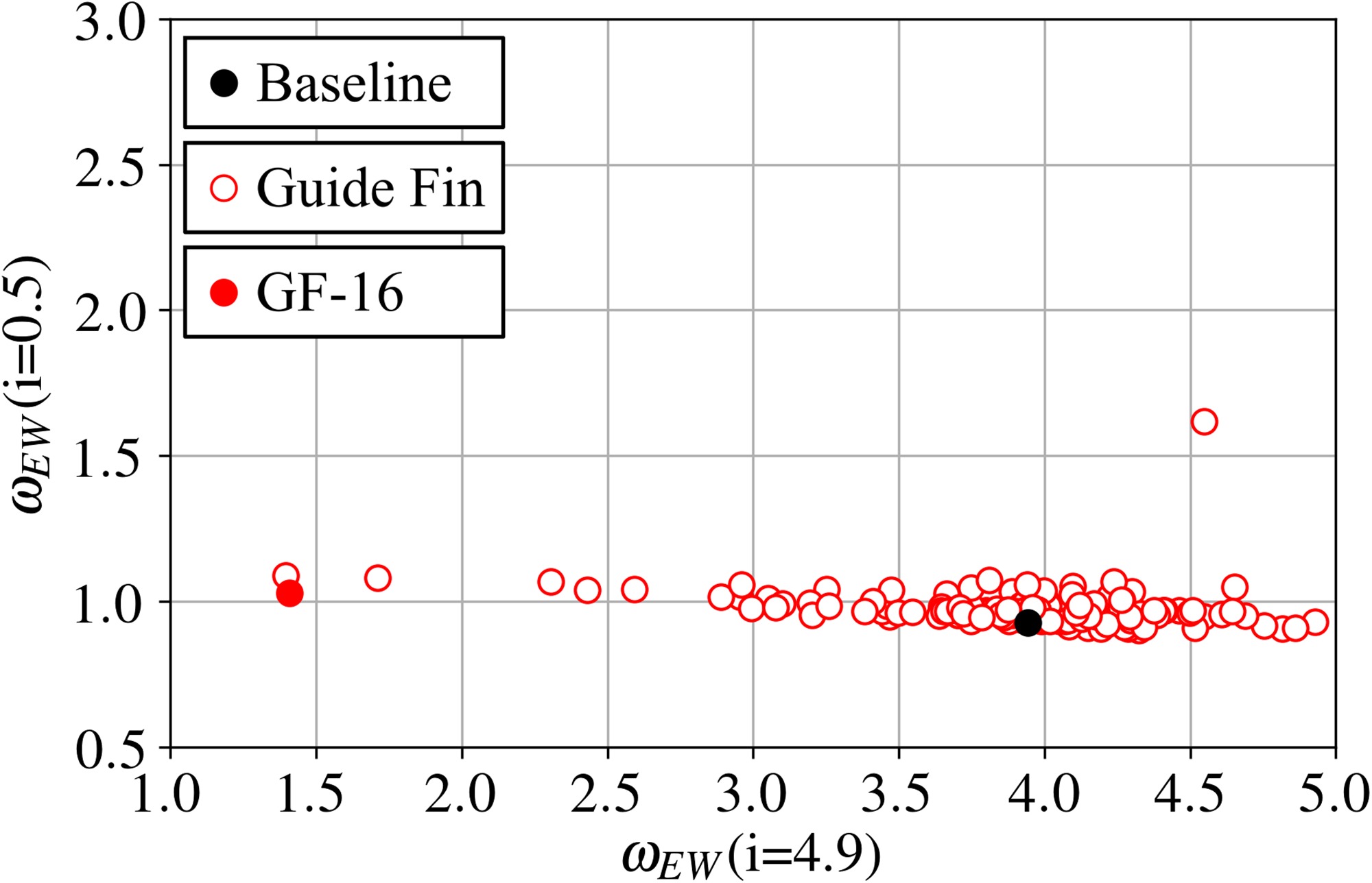
Results of DOE-4 show a widely spread cloud of points with guide fins that either deteriorate or improve the flow. No guide fin improves the flow on both objective functions compared to the baseline configuration, but several configurations dominate the others, in the Pareto sense. GF-4, in green, is particularly of interest as it significantly decreases the losses at high incidence without deteriorating too much the flow near design. Most of guide fins of the DOE-16 have a relatively low impact on the losses at near-design. This is consistent with its related design space, in which guide fins are forced to be relatively aligned with the local stator camber line. However, they are spread across a large range of losses at i = 4.9°. For the same reasons as GF-4, GF-16 appears to be particularly interesting.

In order to assess the ability of this RANS-based set up to find efficient guide fins with two different parametrisations, GF-4 and GF-16 are selected for experimental investigations.

Experimental validation

Table 4 gathers the experimental and RANS evaluations of GF-4 and GF-16. Experimental results confirm that both reduce or have a negligible effect on the endwall losses at 0.5°, and strongly reduce these losses at 4.9°. Notably, a maximum relative loss reduction of 36% is measured with GF-4. DOE-4 and DOE-16 thus enabled to find interesting guide fins that lower the losses. However, these guide fins appear less performant at 4.9° than expected.

GF-16 is evaluated on more incidences for a more in-depth characterisation. Results are gathered in Figure 14. It appears that endwall losses are predicted to increase smoothly with the incidence. RANS predictions thus do not exhibit a critical incidence anymore, yielding an understandable over prediction of the gain in losses. Moreover, experimental endwall losses are decreased not only at 0.5° and 4.9°, but on a broad range of incidence from 0° to 5.9°. Notably, a net gain of 2.06%, corresponding to a relative gain of 47% is found experimentally at 5.4°, the last incidence before the midspan profile starts separating. GF-16 thus improves the robustness to stall while not degrading near-design losses.

Figure 14.

Evolution of the endwall losses on the measurement plane. Baseline Vs GF-16.

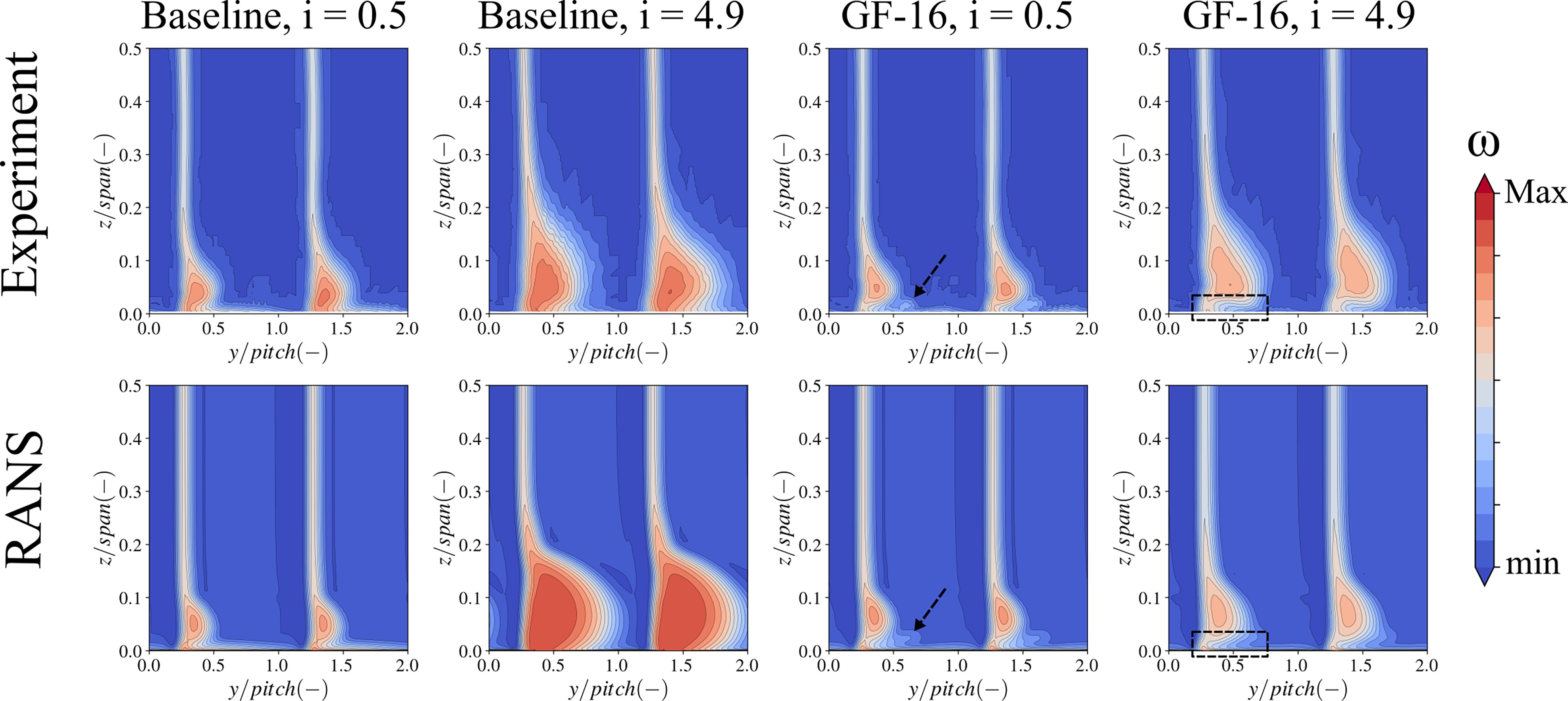
Figure 15 compares the loss distributions predicted by RANS and measured downstream of the cascade, with and without guide fin at 0.5° and 4.9°. In the baseline case, RANS is found to under predict the corner separation at 0.5° and to over predict it at 4.9° with respect to experimental results. However, its spatial extension seems well captured. This is typical of a flow evolution before and after the critical incidence. On the other hand, predictions with GF-16 do not exhibit such an over prediction at 4.9°. This is consistent with the smooth evolution of the endwall losses and the absence of critical incidence in that case. Moreover, specific loss patterns are retrieved, such as the low loss region framed in black at 4.9° and the signature of the guide fin tip vortex pointed out by the black arrow at 0.5°. This confirms that the refinement levels in the experimental probe mesh and the numerical hybrid mesh are consistent with one another.

Figure 15.

Total pressure losses on the measurement plane 0.2c downstream of the cascade. Black rectangle: low loss region. Black arrow: signature of guide fin tip vortex. The investigated blade is on the left.

The implemented numerical methodology enabled to find interesting guide fins, using RANS predictions on two incidences. Adding a guide fin that reduces the losses is found to improve the prediction of the loss distribution downstream of the cascade. Therefore, the use of RANS is proven legitimate for finding efficient guide fins. Beyond the scope of this work, RANS seems promising for an optimisation process, in which the influence of more efficient guide fins could be better predicted.