mGT dynamic model

The mGT dynamic model developed for and described in this paper, aims at simulating the behaviour of the Turbec T100 engine which is located at Vrije Universiteit Brussel (VUB). This mGT, exploiting the recuperated Brayton cycle can operate in dry and wet modes as it was converted into a micro humid air turbine (De Paepe et al., 2014). For the purposes of this paper, we are only concerned with the dry mode simulation. The T100 has a nominal power output of 100 kWe, 165 kWth with a maximal rotational speed close to 70,000 rpm at nominal operating conditions. It is equipped with a control system that keeps the produced electric power constant by adjusting the rotational speed. Moreover, Turbine Outlet Temperature (TOT) is also controlled and fixed at around 645°C by managing the fuel flow in the combustion chamber to maintain high thermal efficiency.

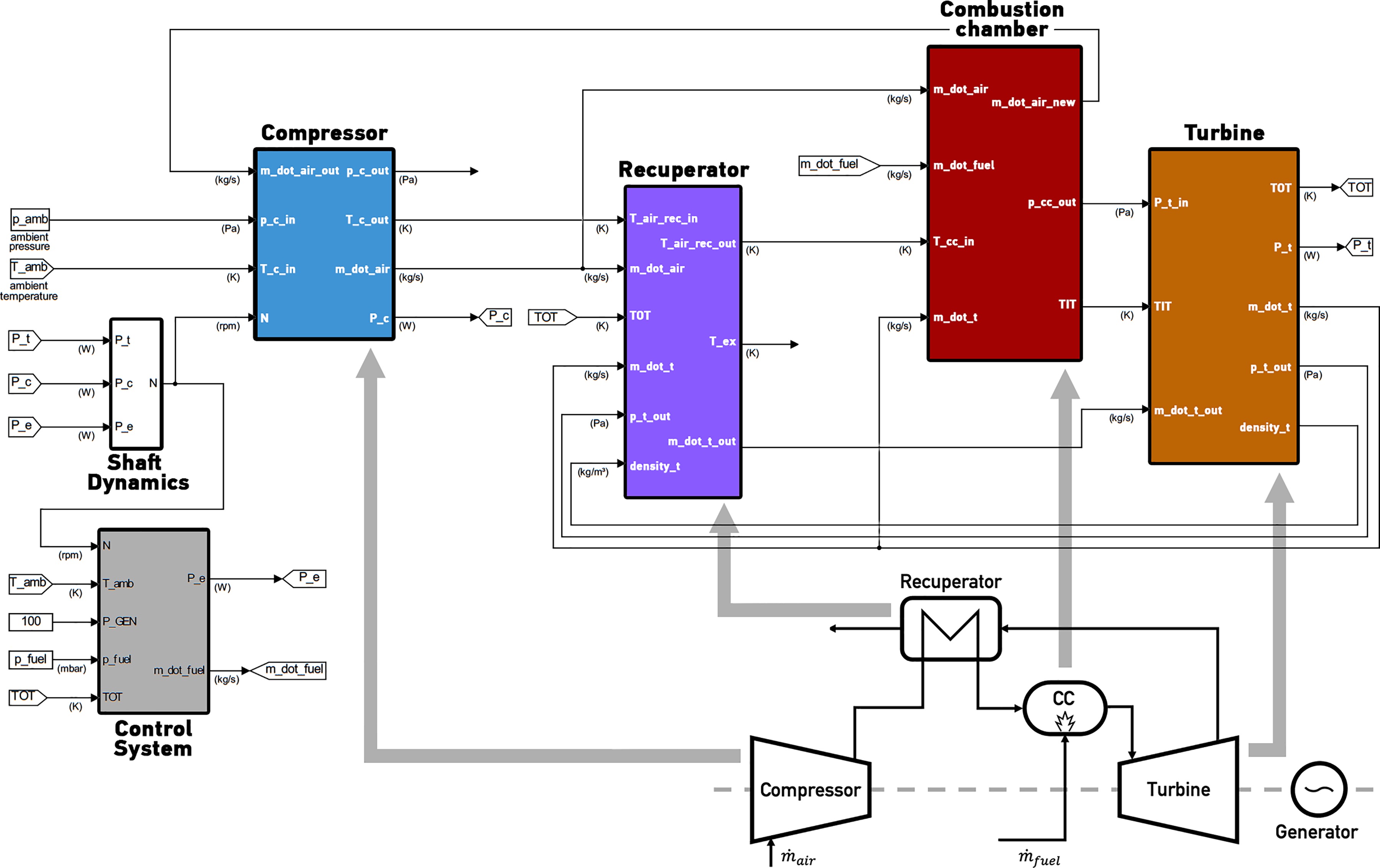
The simulation tool is coded in MATLAB/SIMULINK environment. It offers the ability to combine different blocks and user-defined functions into a subsystem as it is depicted in Figure 1. In all cycle components, we pursued a 0-D modelling with a lumped parameter approach to account for the energy and mass conservation dynamics (Traverso, 2005). The control system consists of the power control which changes the produced power to achieve the desired speed and the fuel control that keeps a constant TOT. The scheme and parameters of the control tool have been received from the manufacturer and are based on a similar approach as described in Montero Carrero et al. (Montero Montero Carrero et al., 2015). For the combustion chamber, we assume a constant volume inside it and a homogeneous air/natural gas mixture. Moreover, a plenum is placed after the instant combustion to account for the pressure and mass flow dynamics.

Figure 1.

Model layout of the mGT cycle.

Turbomachinery map fitting

The purpose of this process is to fit the accessible map data with a specific mathematical equation for both turbomachinery (compressor and turbine) component performance maps. For instance, the fitting equation for each compressor map iso-speed line should have a single form that is controlled by the coefficients of the equation. The map data of the T100 mGT, used for this study, is provided by the manufacturer. Therefore, the precision of our fitting techniques relies on the deviation from the data and the form of the mathematical equation. For this reason, 3 fitting cases will be analysed for both compressor and turbine maps and tested and the technique that minimizes the error from the data will be integrated into the dynamic model.

Compressor map

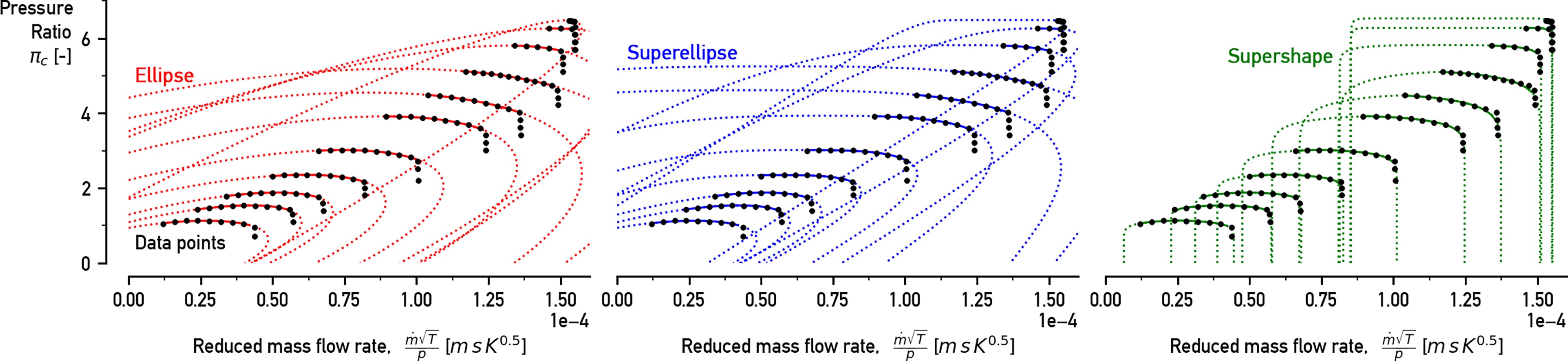
For the representation of pressure ratio πc in relation to the reduced mass flow m˙c rate and shaft speed N, three fitting curves are tested with different complexities. The equations of the three cases are presented below.

(1)

Ellipse:|m˙ccos⁡ϑπc−πcsin⁡ϑπcaπc|2+|m˙csin⁡ϑπc+πccos⁡ϑπcbπc|2=1

(2)

Superellipse:|m˙ccos⁡ϑπc−πcsin⁡ϑπcaπc|n+|m˙csin⁡ϑπc+πccos⁡ϑπcbπc|n=1

(3)

Supershape:|m˙c−x0πcaπc|n1+|πcbπc|n2=1

Equation 1 is an ellipse curve with a center at (0,0) and axes rotation. The Superellipse is a curve with the same parameters as the Ellipse and a coefficient n which alters the shape and adds an extra degree of freedom. For equation 3, a Supershape curve is used with a center at (x0,0), 5 degrees of freedom and no axes rotation. The fitting of the several speed lines for the three cases is presented in Figure 2. It is easily observed that Ellipse and Superellipse are not able to simulate the steep decrease in pressure ratio (choking conditions). Hence, the Supershape is employed to test if we can fit the data points in that region with a single equation. It seems that this equation can fit all the data points but with questionable accuracy. Therefore, we calculated the relative Root-Mean Squared Error (RMSE) for each case in every speed line of the data points that do not belong to the choking region and compared the different methods. Figure (a) shows that Ellipse has the most effective fitting behaviour in low as well as high rotational speeds with a relative error below 0.9%. Moreover, Supershape presented increased error (above 1.5%) despite the fitting of all data points. Therefore, Case 1 is chosen to model the speed lines due to its satisfactory results among the proposed fitting methods. This technique is also coupled with a linear interpolation between the points of maximum mass flow and minimum pressure ratio at the chocking region to account for the accurate representation of the steep decrease in the πc value. Then, the parameters of the adopted equation (α,b,ϑ) are expressed as a function of rotational speed with the use of 1-D interpolation function provided by Python programming language.

Figure 2.

Compressor maps fitting approaches: Ellipse, Superellipse and Supershape.

Turbine map

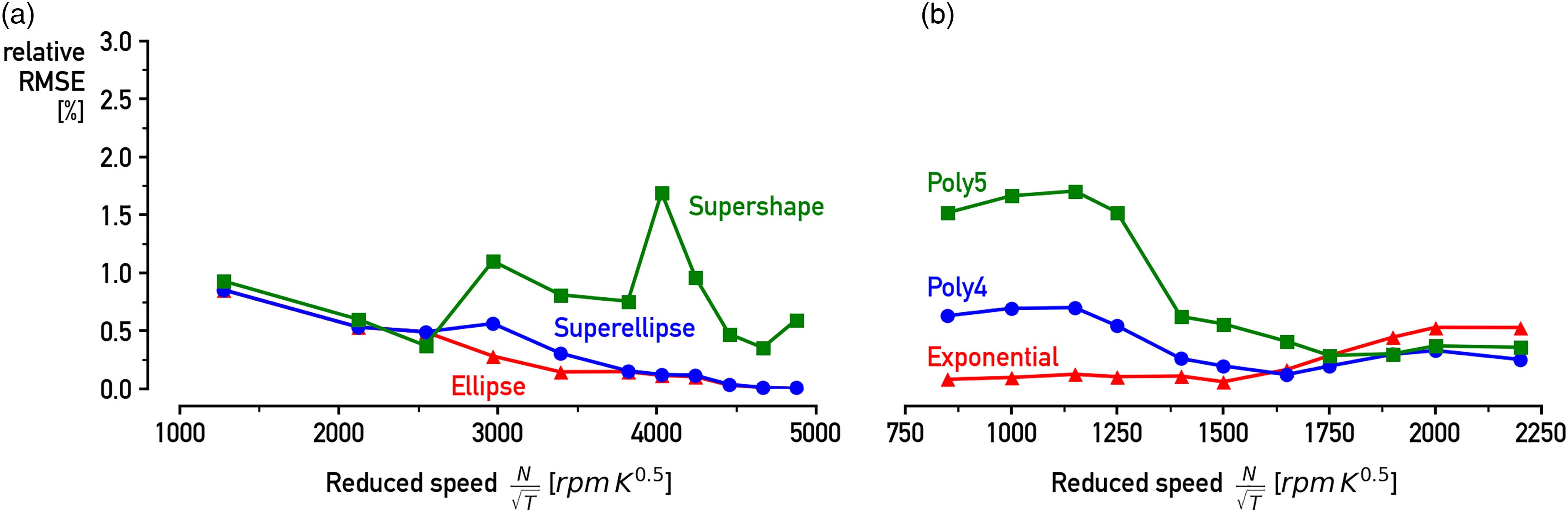
A comparable approach is followed for the turbine map fitting. Although for this occasion a different group of fitting curves is applied. Due to the distinct form of the iso-speed lines in a turbine map, an exponential curve with a rotating axis is used (equation 4). The fitting behaviour for his equation is depicted in Figure 3 and is compared with a 4th and 5th degree polynomials that are the equations 5 and 6 consequently.

Figure 3.

The Exponential fitting approach shows good fitting characteristics on the data points of the turbine map.

(4)

Exponential:m˙tcos⁡ϑ−πtsin⁡ϑ=b(πtcos⁡ϑ−m˙tsin⁡ϑ+a)+c

(5)

Poly4:m˙t=a⋅πt4+b⋅πt3+c⋅πt2+d⋅πt+e

(6)

Poly5:m˙t=a⋅πt5+b⋅πt4+c⋅πt3+d⋅πt2+e⋅πt+f

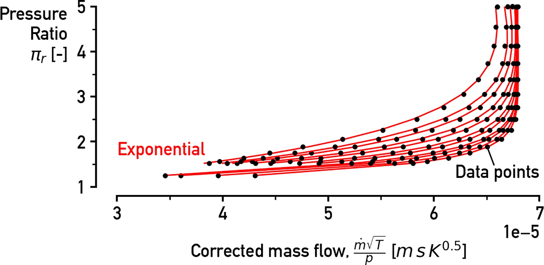
Exponential has 4 coefficients (α,b,c,ϑ) and its fitting behaviour on the datapoints is shown in Figure 4. This equation can only be solved indirectly, contrary to the other two cases. This characteristic makes it computational heavier solution against polynomial curves. However, in Figure 4(b) we can see that equation 4 presents exceptional fitting accuracy, especially in the low-speed region. For this reason, again a hybrid scheme was adopted for the turbine map fitting. Thus, the Exponential equation is employed for the low-speed region (N<1750rpmK0.5) and Poly4 for the rest to ensure a balance between accuracy and fast calculations. Additionally, the coefficients of the adopted curves are demonstrated as a function of rotational speed with 1-D interpolation. Similar methods and fitting equations were used for the calculation of the efficiency curves for both the compressor and turbine (not included in this work).

Figure 4.

The relative RMSE of the 3 cases as a function of the reduced speed for (a) the compressor and (b) the turbine map fitting. The relative RMSE of the fitting curves for the compressor and turbine highlight the superiority of the first method (red lines).

1-D heat exchanger model

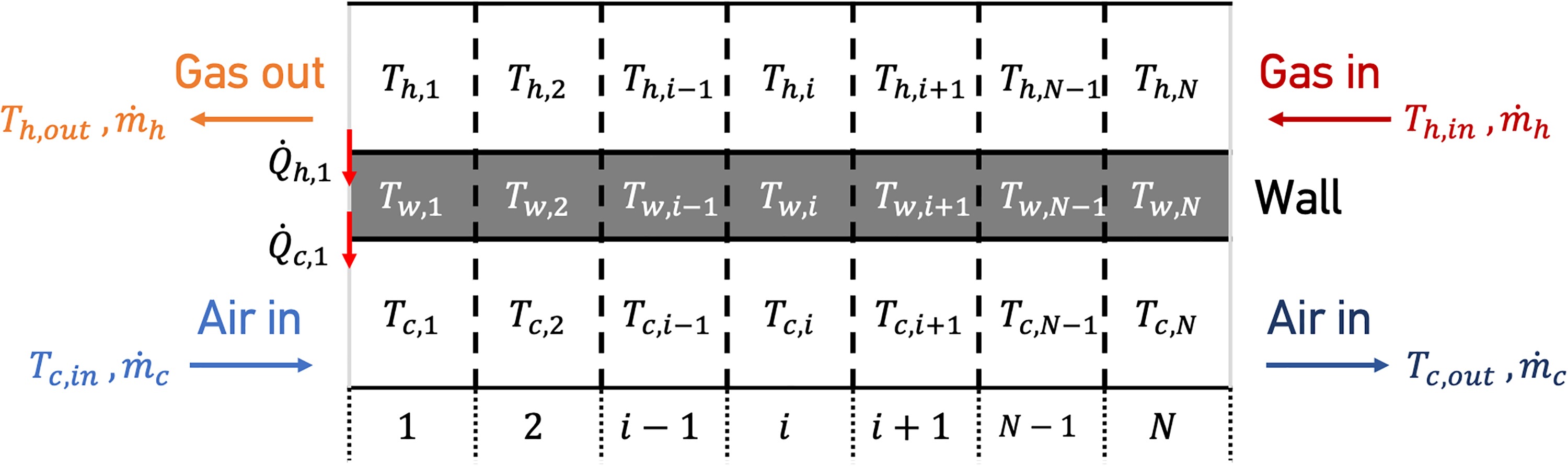
The current work focuses on the recuperator developed by RSAB and specifically designed for mGT applications (Lagerström and Xie, 2002). Such a 1-D model is necessary as a simpler 0-D approach assumes a constant wall temperature inside the heat exchanger. This creates numerical problems in dynamics conditions and especially in compact recuperators used for mGTs where the temperature wall gradient is high (McDonald, 2003). The heat exchanger is discretised into a N cells (5 cells used for good accuracy) according to Figure, where the energy equation is applied using the following equation:

The heat capacity and the mass of the casing are expressed with c_m and m respectively. The remaining values of the equation are presented in Figure 5. For the heat balance of the air and gas stream, we applied a steady-state approximation. This is fairly justified as the temperature rate of change in each “stream” cell is greater than the temperature rate of change in each “wall” cell. So, the heats that are absorbed and released in each cell are presented below:

Figure 5.

Modelling scheme of the heat exchanger.

We also assumed that the thermal resistance of the recuperator plates is fairly small and could be ignored.

Moreover, two different cases for the heat transfer coefficient will be considered. In the first one, the UA is kept constant and is taken by the work of Lagerström at nominal conditions. In the second case, the UA is expressed as a function of m˙c. This function is constructed by tuning the UA in order for the component to match the effectiveness (ε) of experimental data of the T100 in 4 different operating points (100, 90, 80, 70 kW). Then a linear interpolation is applied between the tuned UA points which have a range between 5,117 and 5,279 W/K.

Map fitting

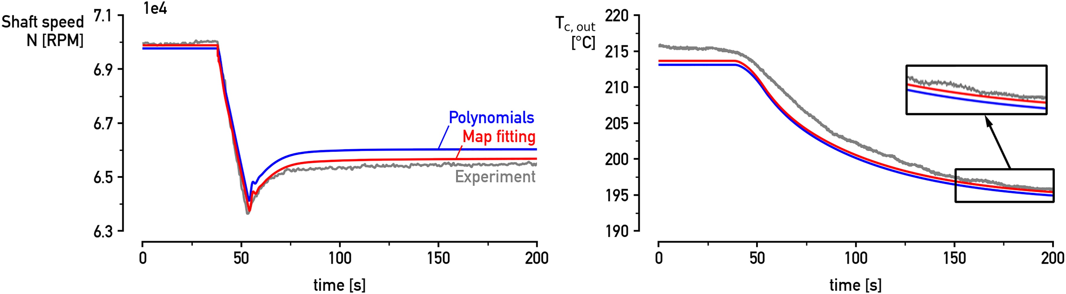
The map fitting technique that is implemented and described above is compared with the approach that is proposed by Sieros et al. (called “Polynomials”) for the compressor and assumes that the turbine is chocked (Sieros et al., 1997). Both methods are considered common in turbomachinery modeling. The rotational speed is closely related to the pressure of the system by the compressor and turbine map. Moreover, the air temperature at the outlet of the compressor is linked with the compressor map through the isentropic law. Hence, Figure 6 shows the response of shaft speed (N) and compressor outlet temperature (Tc,out) and their difference from the experimental data at a load step −20 kWe from the nominal power (100 kWe). The rotational speed behaviour shows a satisfying agreement with the experimental data. The transition to lower rotational speed is modeled effectively as the simulation follows the slope of the experimental data rather well. Furthermore, the deviation from the real shaft speed at 100 and 80 kWe (in 0 and 200 s respectively) is reduced by the implementation of the “Map fitting” method as the “Polynomials” approach has a larger relative mean error (1.15% and 0.38% respectively). Similarly, Tc,out satisfactorily follows the experimental data for the demanded power step. The accurate simulation of this value is crucial as a deviation from the measured data can propagate to the recuperator component. This will prevent us from accurately validating the heat exchanger 1-D model. Therefore, as shown in Figure 6, Tc,out presents a maximum difference in nominal power of no more than 1°C. Also, the results tend to match those from the experiment at 200 s. The “Polynomials” model, in this case, shows very close values with our method. This is explained as the temperature is more dependent on the connected “lumped volume” in dynamic conditions than the pressure ratio. Moreover, the variation in the steady-state value of Tc,out at nominal power is caused by the assumption of constant pressure losses inside the compressor.

Figure 6.

The behaviour of Rotational speed and Temperature in the compressor outlet for a demanded electrical power output step from 100 to 80 kWe.

Recuperator model

As it was described in the previous section, the heat exchanger model is initially developed with a constant heat transfer coefficient taken at nominal conditions. This approach was tested and it seemed more appropriate to use a variable UA in order to capture the temperature dynamics inside the heat exchanger with precision. Therefore, experimental data from the T100 were utilized and we calculated the effectiveness (ε) of the component in four different operating modes (70, 80, 90 and 100 kWe). Then the UA is tuned until the model simulates the effectiveness that was observed from experiments in those operating modes.

Figure 7 shows the behaviour of the recuperator outlet temperature (Tcc,in) with negative steps in the demanded electrical power. The transition from 100 to 90 kWe (Figure 7a) presents a small deviation in the steady-state values from the experimental data. This absolute difference is approximately 1°C at 500 s and is a product of the constant UA. In dynamic operation the specific heat flux (q˙) along with the temperature difference between the wall and the fluid (ΔT) change. As a result, UA does not remain constant from a physical point of view. Thus, the 1-D model slightly miscalculates the Tcc,in during the transition to 90 kWe. We easily overcome this problem by using a variable UA being a function of the mass flow of the cold medium and tuning it to simulate the ε that was observed from experiments in each operating point. After the introduction of a variable UA the Tcc,in follows satisfactorily the experimental data in the two load steps of Figure 7. Moreover, the transition curve in 50–100 s is faithfully followed in both Figure 7a and b by the model.

Figure 7.

The calculated recuperator outlet temperature (cold side) follows well the experimental data for a step in demanded electrical power output after tuning from (a) 100 to 90 kWe and (b) 100 to 80 kWe.

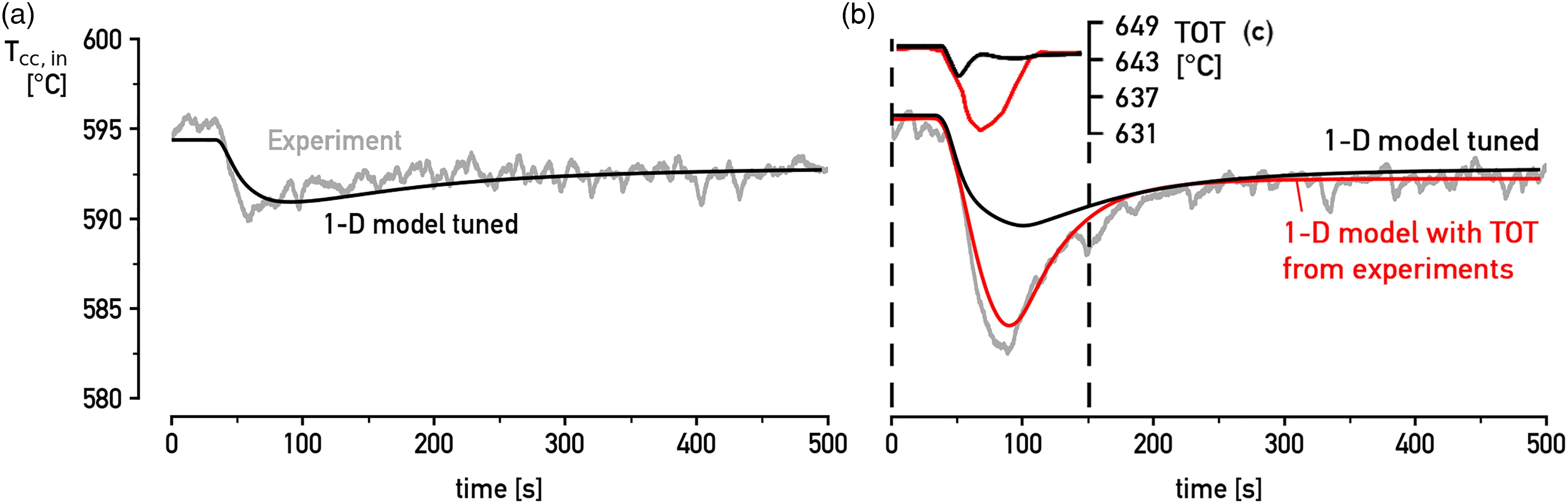
Figure 8a shows that after the 1-D model is tuned, the deviation for the experiments is minimized in a positive load step-change as well. This is observed in Figure 8b. Although, in this case, the model cannot simulate efficiently the large drop in temperature at the time period of 50–150 s. This problem is not truly related to the features of the 1-D numerical model. This steep decrease in the temperature of the experimental data is caused by the drop in TOT and it is the product of the control system of the test rig. During the experimental tests, the demanded power is stabilised first and afterwards the TOT is manipulated to remain constant. A positive step-change in the demanded power leads to an increase in the mass flow rate of the engine. As a result, the mixture in the combustion chamber becomes leaner and the Turbine Inlet Temperature (TIT) decreases along with the TOT. This drop in TOT cannot be properly calculated by the mGT dynamic model as the model's control system tries to immediately stabilize the TOT at 645°C. Therefore, this behaviour can be fixed by adjusting the characteristics of the control system model. As it is depicted in Figure 8c the TOT of the measurements drops substantially compared with the simulated TOT. The effect of this phenomenon in the Tcc,in is observed when we use the TOT from the measurements as an input in the model (Figure 8b red lines). As the TOT drops, the simulated Tcc,in is affected as well and gets closer to the experimental data. Thus, it is clear that the model simulates the recuperator performance with good precision. The effect of the control system on the design parameters is not part of the current work due to space limitations. However, it seems crucial to focus on the behaviour of the control in future work.

Figure 8.

Recuperator outlet temperature (cold side) for a step in demanded electrical power output from (a) 90 to 100 kWe and (b) 80 to 100 kWe.