
Introduction
The fast uptake of renewable sources in power generation in the recent years has aggravated the problem of flexibility of conventional power generation systems. The intermittent nature of the renewable sources (solar and wind in particular) imposes new operational challenges for power plants which will be required to ramp more often with frequent shut-downs and start-ups. During the shut-down regimes, the turbine casing components are exposed to the buoyant flows with pure natural and mixed convection, which then lead to non-uniform cooling due to temperature non-uniformity on the components. Consequently, the non-uniform cooling rates may cause severe fatigue on the casing.
Considering these challenges, the first step towards addressing the issues would be ensuring that the flow physics during the shut-down regimes are thoroughly investigated. The experimental investigations, however, are often not feasible since the direct measurements in the flow field in the turbine cavities are not trivial. Therefore, majority of the observations heavily rely on computational methods. Although a large body of literature has sought to provide experimental data for pure natural (for example Beckmann (1931), Liu et al. (1961), Grigull and Hauf (1966), Kuehn and Goldstein (1976), and Fahy et al. (2018)) and forced convection (Brighton (1963), Farias et al. (2009) and Hosseini et al. (2009) among others), mixed type of convection in the turbine casing cavities has not been previously assessed to a broad extent. The experimental investigations concerning the mixed type type of flows have been mostly on fully developed duct and pipe flows (for example Kotake and Hattori (1985), Ciampi et al. (1987) and Mohammed et al. (2010)). In the recently conducted research of Murat et al. (2021), a unique experimental facility has been designed and commissioned for mixed type of flows in turbine casing cavities during shut-down regimes, and also incapabilities of Reynolds-averaged Navier-Stokes (RANS) in predicting these type of flows have been highlighted by demonstrating the inadequacy of isotropic turbulence assumption.
The unavailability of the extensive experimental data, in return, ultimately reduces the confidence in the numerical results, which hinders the design optimization and the advance turbulence modelling development for the mixed type of flows.
Experimental methodology
Background
Mixed type of convection occurs in a wide range of turbomachinery applications, and are therefore of great importance. As mentioned earlier, especially high pressure (HP) steam turbine casing is exposed to both natural and mixed convection during shut-down regimes with different operating conditions. The cavity formed by the inner and outer turbine casings could be considered as a horizontal concentric annulus as seen in Figure 1 where various flow regimes taking place in the casing cavity are also presented.
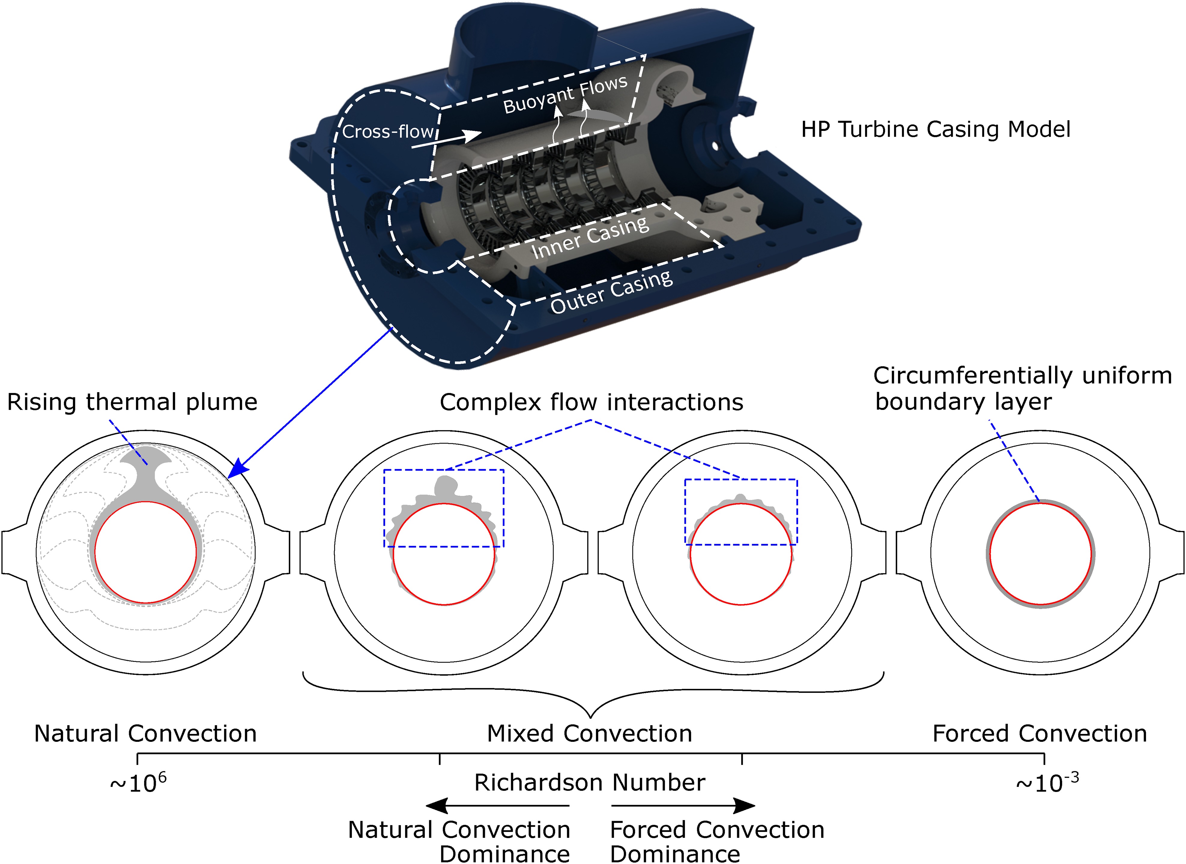
In the case of pure natural convection, thermal plume occurs at the top of the heated inner cylinder, which rises and impinges on the outer casing. This leads to a non-uniform cooling. After impingement, the fluid cools down and moves down the lower portion of the annulus where the flow tends to be stable. When the pure forced convection takes places, a circumferentially uniform boundary layer forms around the inner cylinder as shown in Figure 1. The flow behaviour in the upper portion of the annulus significantly changes when both natural and forced convection take place simultaneously. The thermal plume region is distorted by the cross-flow, and multiple longitudinal structures develop due to the complex flow interactions.
Experimental facility
An experimental facility illustrated in Figure 2 has been designed for the detailed investigations of mixed (natural and forced) convective type of flows in a simplified turbine casing cavity represented by a horizontal concentric annulus. The inner casing temperature is kept constant by a PID controller at a set value, while the incoming air speed is varied by an industrial blower at the outlet for different mixed convection rates. Low conductivity calcium silicate inserts are used at both end of the inner cylinder, which is made of copper, to minimise the heat loss. Self-adhesive ceramic heat shields have been placed around the outer casing cylinder to reduce the heat dissipation. The facility consists of various measurement ports distributed axially and circumferentially. Measurement locations on the test facility are depicted in the facility schematic in Figure 3 and some of the essential dimensions are tabulated in Table 1. The detailed design information regarding the experimental facility can be found in the study of Murat et al. (2021).
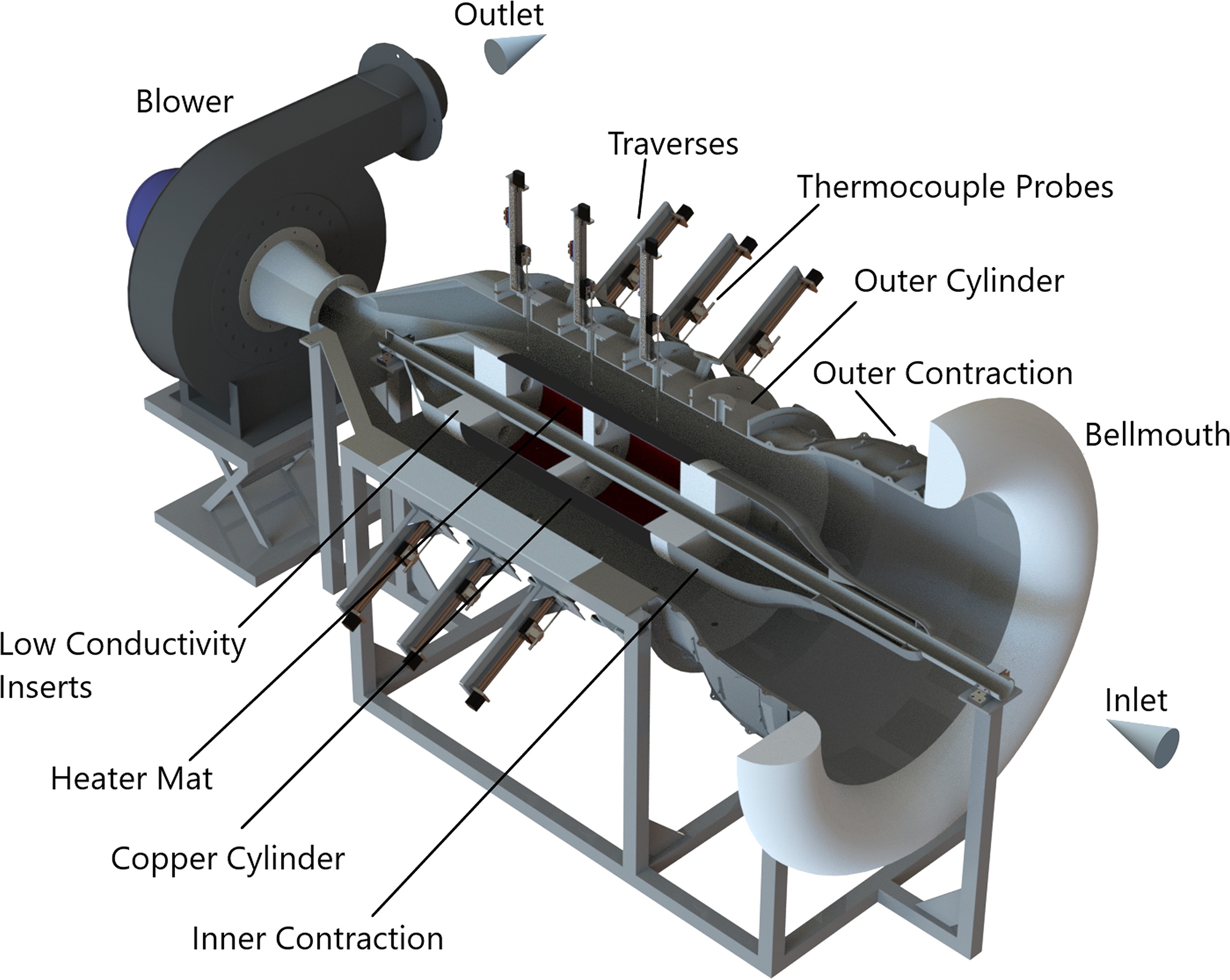
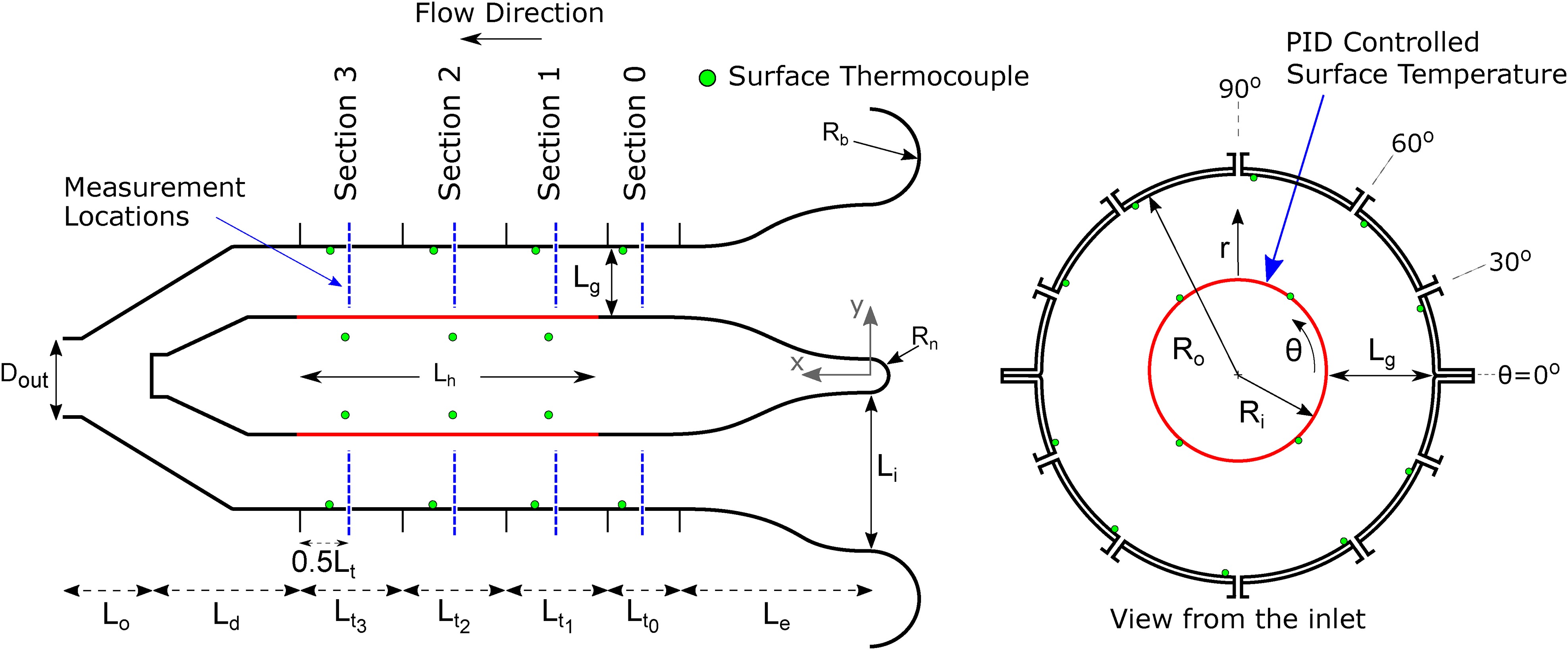
Table 1.
Rig dimensions.
| Parameter | Dimension (mm) | Parameter | Dimension (mm) | Parameter | Dimension (mm) | Parameter | Dimension (mm) |
|---|---|---|---|---|---|---|---|
| 180 | 70 | 720 | 425 | ||||
| 400 | 440 | 250 | 390 | ||||
| 150 | 220 | 300 | 200 |
For pure natural and forced convective flows, Grashof and Reynolds numbers are important non-dimensional parameters to determine the flow regime. Richardson number is used when both natural and forced convection take place simultaneously. The non-dimensional numbers used in the present study are given in Equation 1.
It is important that a test facility is able operate at real engine representative conditions to have realistic conditions. In the present study, the test facility is capable of operating at various mixed convective flow regimes as well as pure natural and forced convective flows. Figure 4 shows the range that the facility can operate in comparison with the real turbine data during a shut-down regime, which indicates that the facility is capable of reproducing engine realistic conditions. In the same figure, mixed type of flow cases that are presented in this paper are also marked, the details of which are tabulated in Table 2.
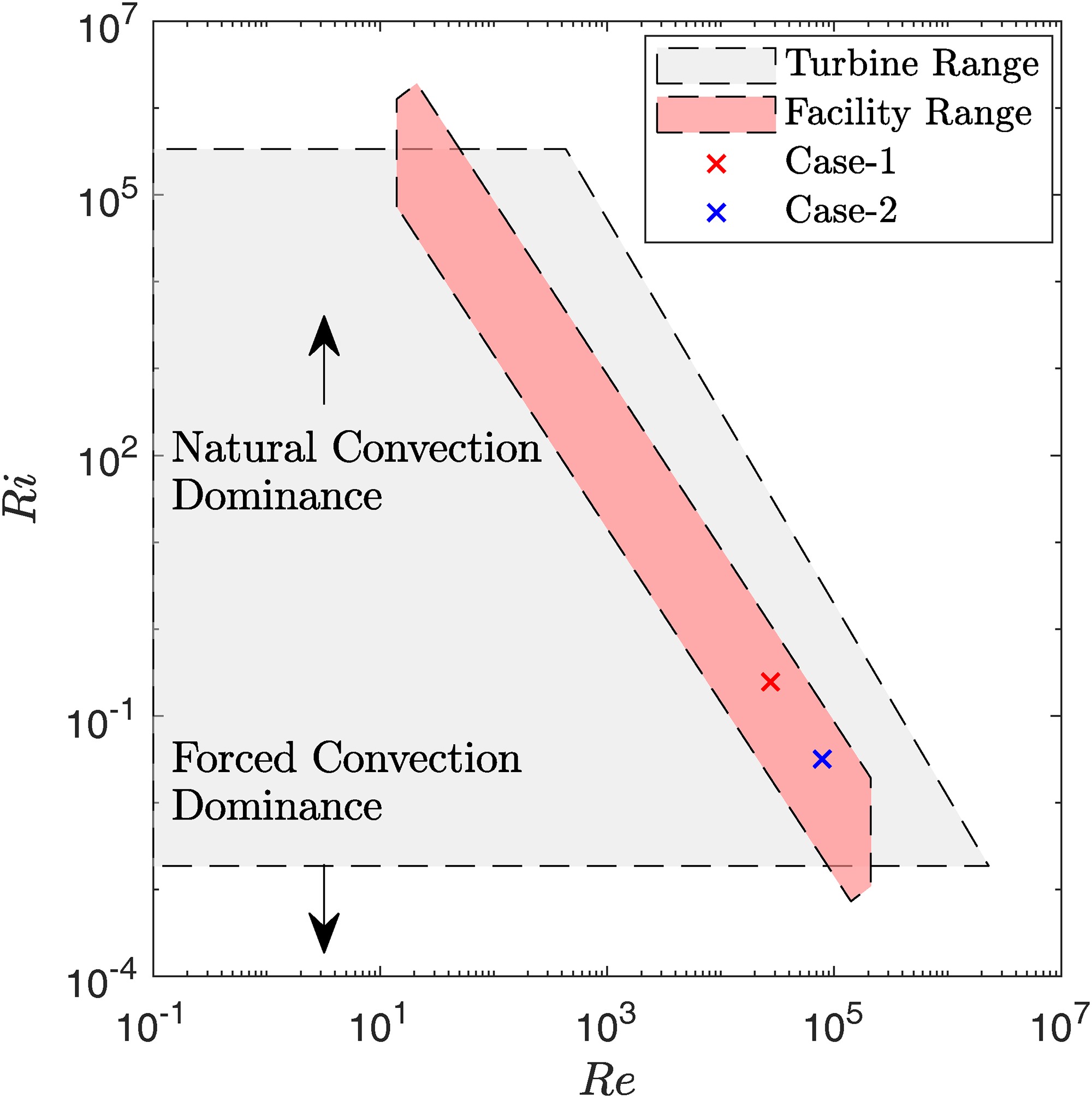
Table 2.
Experiment characteristics.
| Parameter | Case-1 | Case-2 |
|---|---|---|
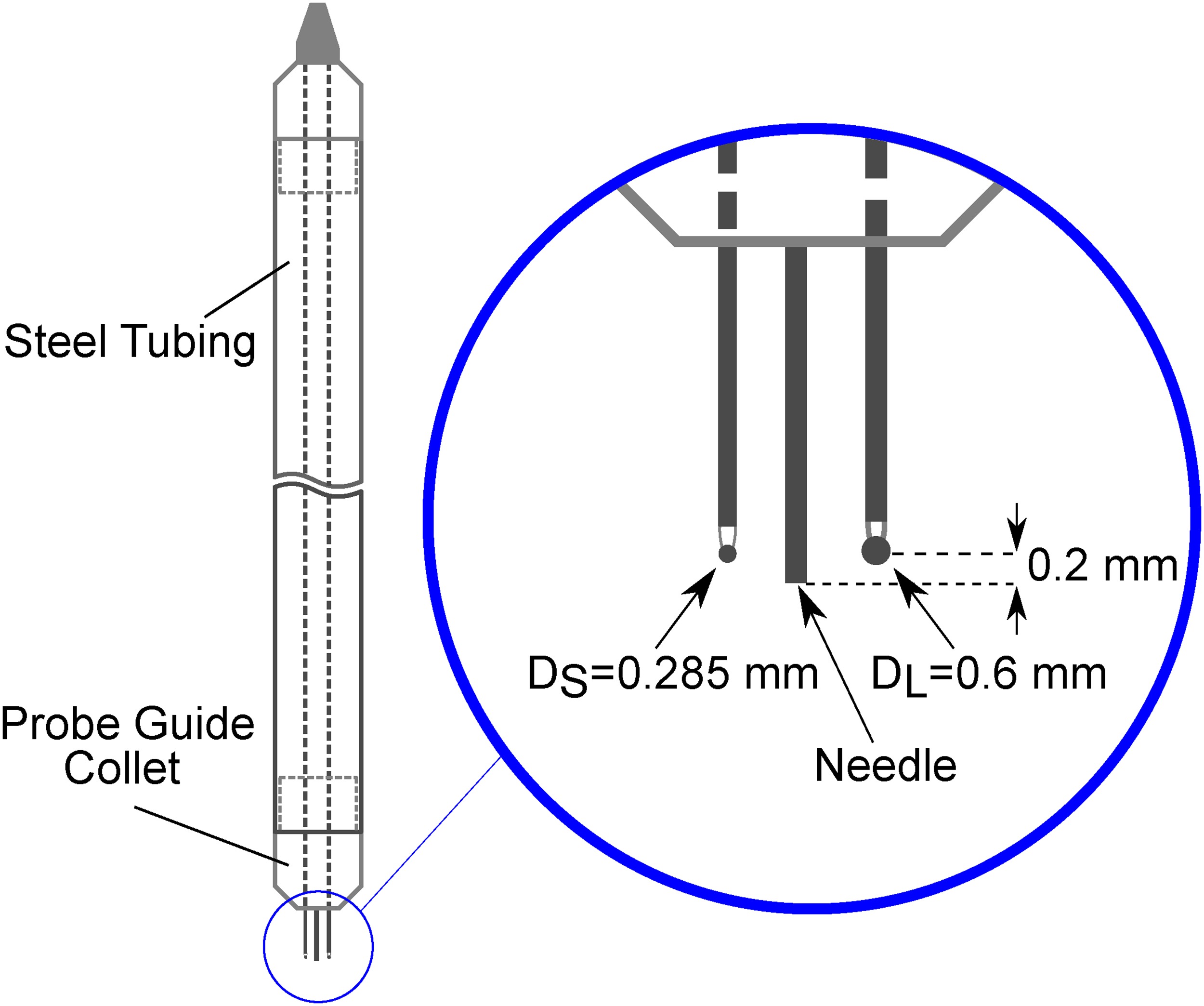
Linear actuators with accuracy of 0.05 mm have been used to traverse the thermocouple probes, which are distributed in axial and circumferential locations. The thermocouple probe houses two K-type thermocouples and a needle to keep the thermocouple beads at a known distance from the heated copper cylinder, as shown in Figure 5. During the measurements, the thermocouple probes were traversed starting from the heated inner cylinder towards the outer cylinder. Step of 0.1 mm was used near the heated wall to be able to capture the near-wall gradients, while relatively larger steps were used away from the walls. Time averaging of unsteady data acquired by National Instruments data acquisition modules was performed over 120 seconds with 50 Hz sampling rate.
Although the heated copper cylinder is covered with a mat black paint, the radiation effect may still be significant. When the heat conduction through the thermocouple sheath tube is ignored, the energy balance applied on a thermocouple bead consists of convective and radiative heat transfer as shown in Equation 2. Measurement or estimation of the effective surrounding temperature,
Numerical methodology
Large Eddy Simulations (LES) have been performed for mixed convection experiments to further investigate the flow field with ANSYS Fluent (ANSYS, 2020). Pressure-velocity coupling is maintained with the SIMPLE algorithm with a segregated manner. Second order scheme has been used for pressure discretisation. A bounded central differencing scheme has been used for momentum and energy. A bounded second order implicit scheme has been chosen for the temporal discretisation. Dynamic Smagorinsky model (Germano et al., 1990) has been employed for sub-grid scale modelling. Large eddy simulations were initialized using the flow field predicted by RANS simulations.
Two conformal structured hexahedral type meshes with 29.6 and 25.3 million nodes have been used for Case-1 and Case-2, respectively. Detailed information on mesh resolutions in wall units is given in Tables 3 and 4.
Table 3.
Case-1 mesh resolution.
| Case-1 | 17.07 | 18.22 | 40.51 | 0.29 | 3.45 | 3.45 | 7.58 | 1.16 | 9.52 |
Table 4.
Case-2 mesh resolution.
| Case-2 | 23.53 | 25.02 | 55.61 | 0.31 | 4.18 | 4.18 | 30.4 | 1.24 | 24.3 |
Time steps of
Table 5.
Fluid properties.
| Case | k (W/mK) | Cp (J/kgK) | Pr | ||
|---|---|---|---|---|---|
| Case-1 | |||||
| Case-2 |
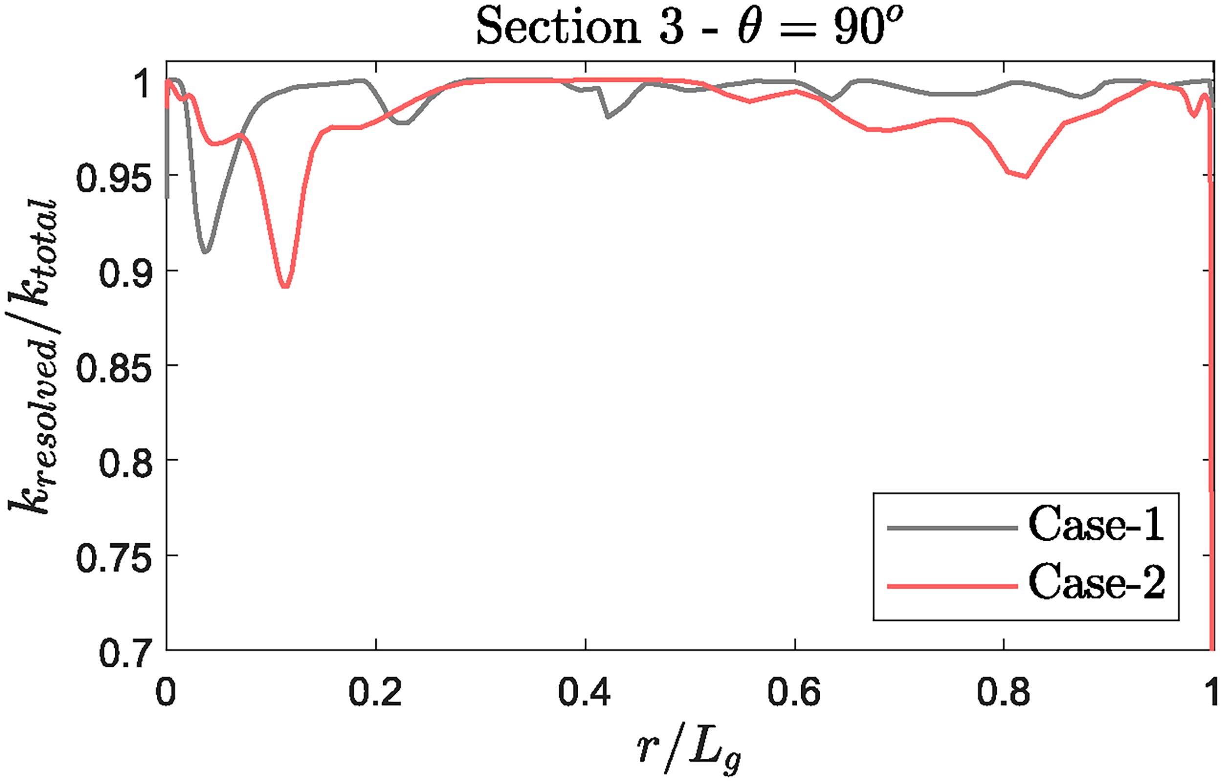
Figure 6 shows the amount of resolved turbulent kinetic energy at Section 3 -

Boundary conditions
The computational domain used for LES is illustrated in Figure 8. As seen in the figure, CFD domain involve a region at upstream of the bellmouth, referred as “entrance region”, to allow boundary layer development over the bellmouth. Mass flow rate for each case has been calculated using the air speed measured at Section 0 by hot-wire anemometry, which read as

Heat transfer measurement and uncertainty analysis
This section explains how the heat fluxes from the heated inner cylinder and the Nusselt numbers are calculated from the raw measurement data in this study. In the viscous sub-layer, the heat transfer occurs only through conduction when the radiation is neglected. Temperature field exhibits the same characteristics as the velocity field (Schlichting and Gersten, 2017). Therefore, the temperature gradient remains linear in the viscous sub-layer, and the heat flux from a solid surface to a fluid can be calculated by Fourier’s law
In the experiments, the temperature gradients were captured using small traverse stepping (0.1 mm) near the heated wall. The near-wall measurement points in the radial direction at each traverse location were fitted to a straight line, and the slope of the each line was used to calculate the heat flux. Fittings were performed using linear regression analysis.
Figure 9 shows the near wall temperature gradient at
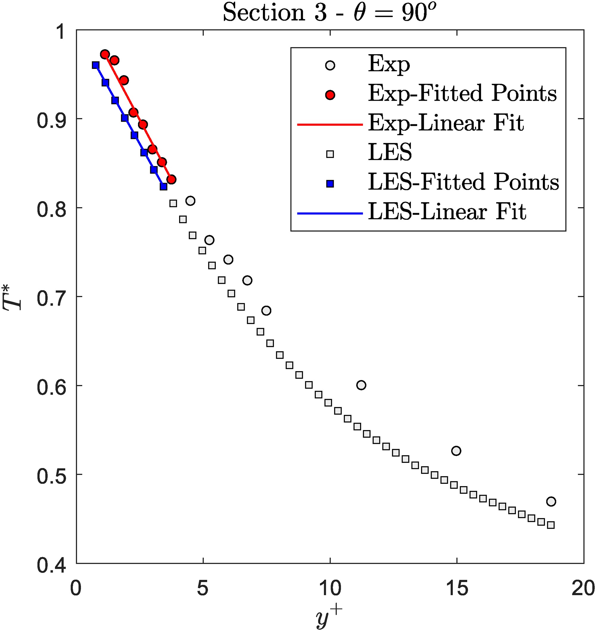
In Figure 10, how the experimentally and numerically calculated Nusselt number varies depending on the end point selection is shown. In order to judge the goodness of the fits,

The experimental heat flux calculation requires detailed analysis at each measurement point since the viscous sub-layer thickness varies around the heated inner cylinder. In addition, the number of points used for line fitting may change remarkably, which consequently leads to the different uncertainties in Nusselt number around the inner cylinder as shown in Figure 11. The associated bias errors for each variable used in Nusselt number calculation are given in Table 7. The uncertainty analysis has been conducted using root sum square method (Moffat, 1988) as shown in Equation 4. The number of points used for the heat flux calculation effects the uncertainty in Nusselt number calculation remarkably since the the heat flux term,

Table 7.
Bias error of each variable.
| Variable | Uncertainty | Variable | Uncertainty |
|---|---|---|---|
| Traverse Thermocouple | Heated Cylinder Diameter | ||
| PID Thermocouple | Traverse |
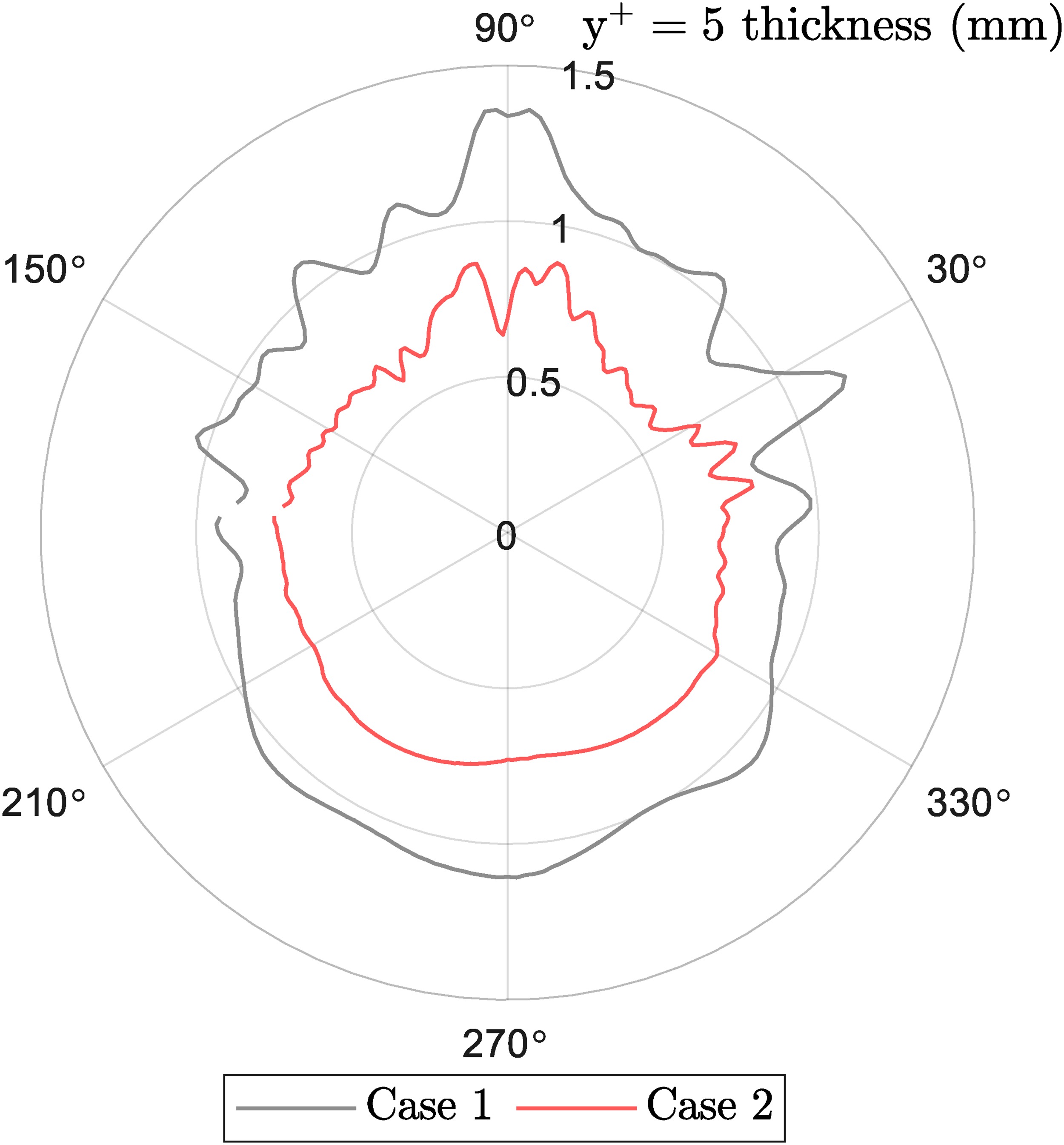
Figure 12 indicates the distance from
Results and discussion
Temperature profiles
Temperature profiles are presented in a non-dimensional form as
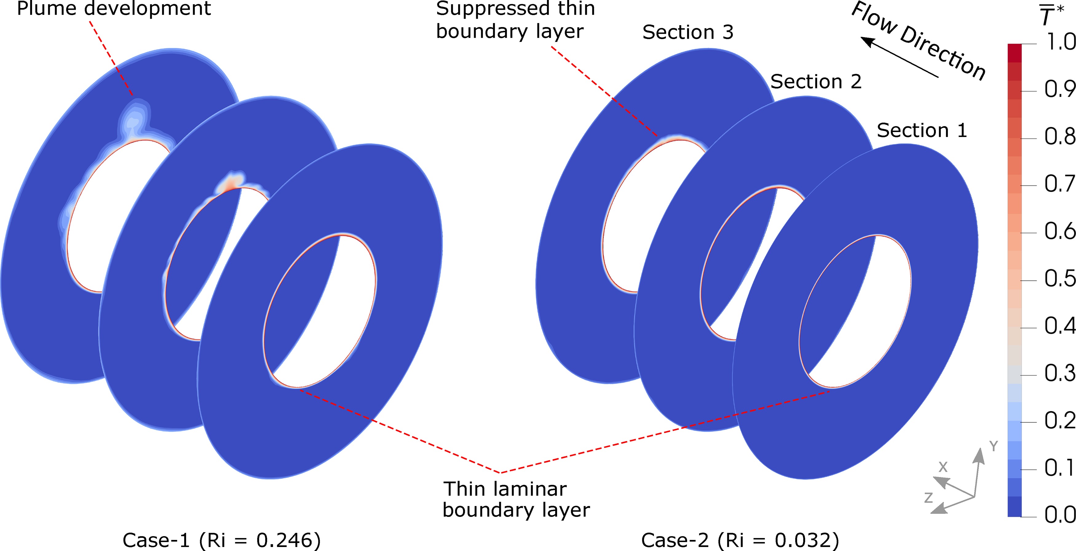
Time-averaged non-dimensional temperature profiles predicted by LES are compared against the experimental data in Figure 14 for Case-1 at Section 1, 2 and 3. At Section 1, the thin temperature boundary layer is present around the inner cylinder, indicating that the buoyancy effect is not strongly pronounced at this section. Good agreement between numerical and experimental results has been achieved at Section 1. As the fluid progresses, the development of the boundary layer becomes noticeably distinguishable at the top of the annulus at
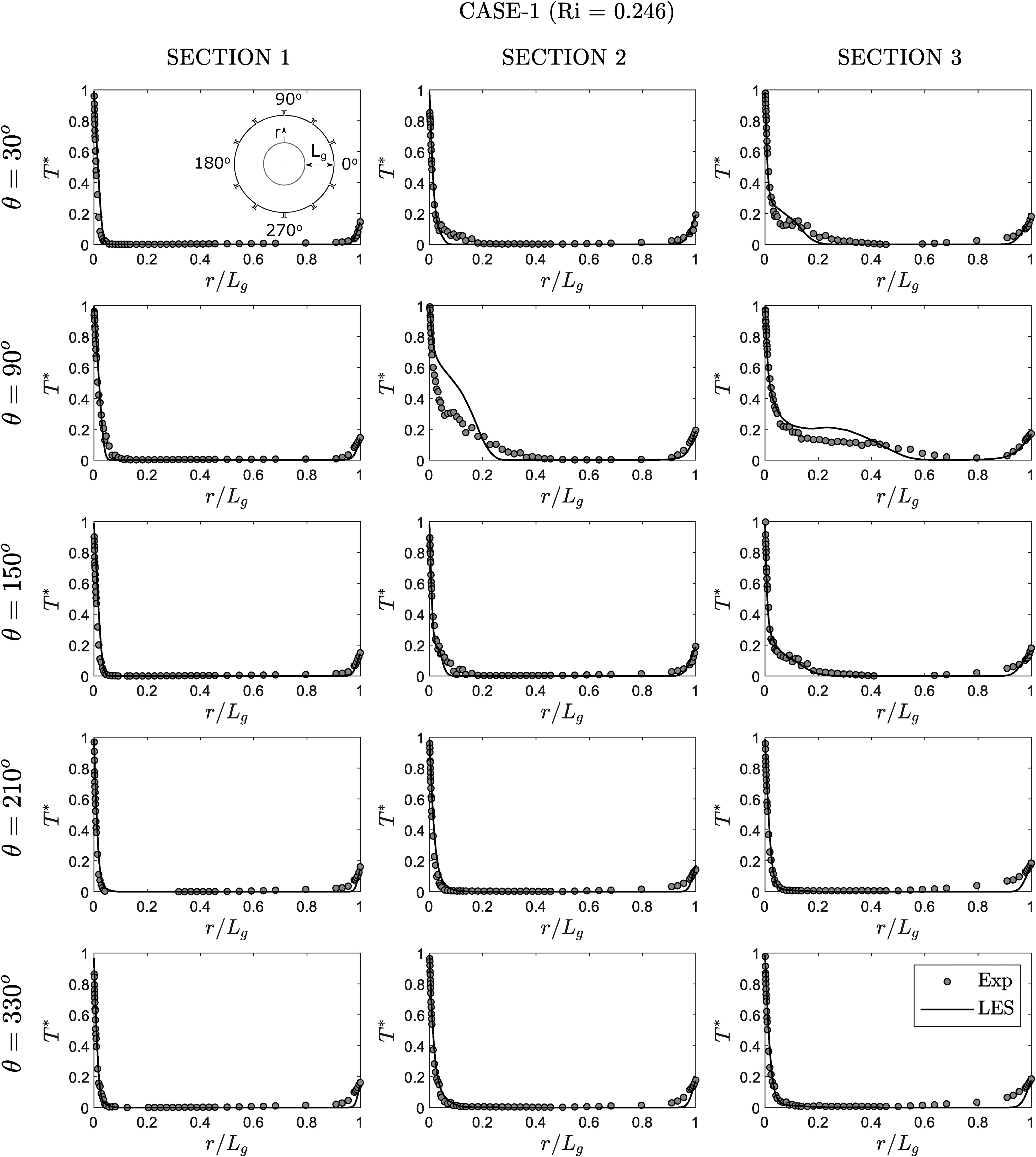
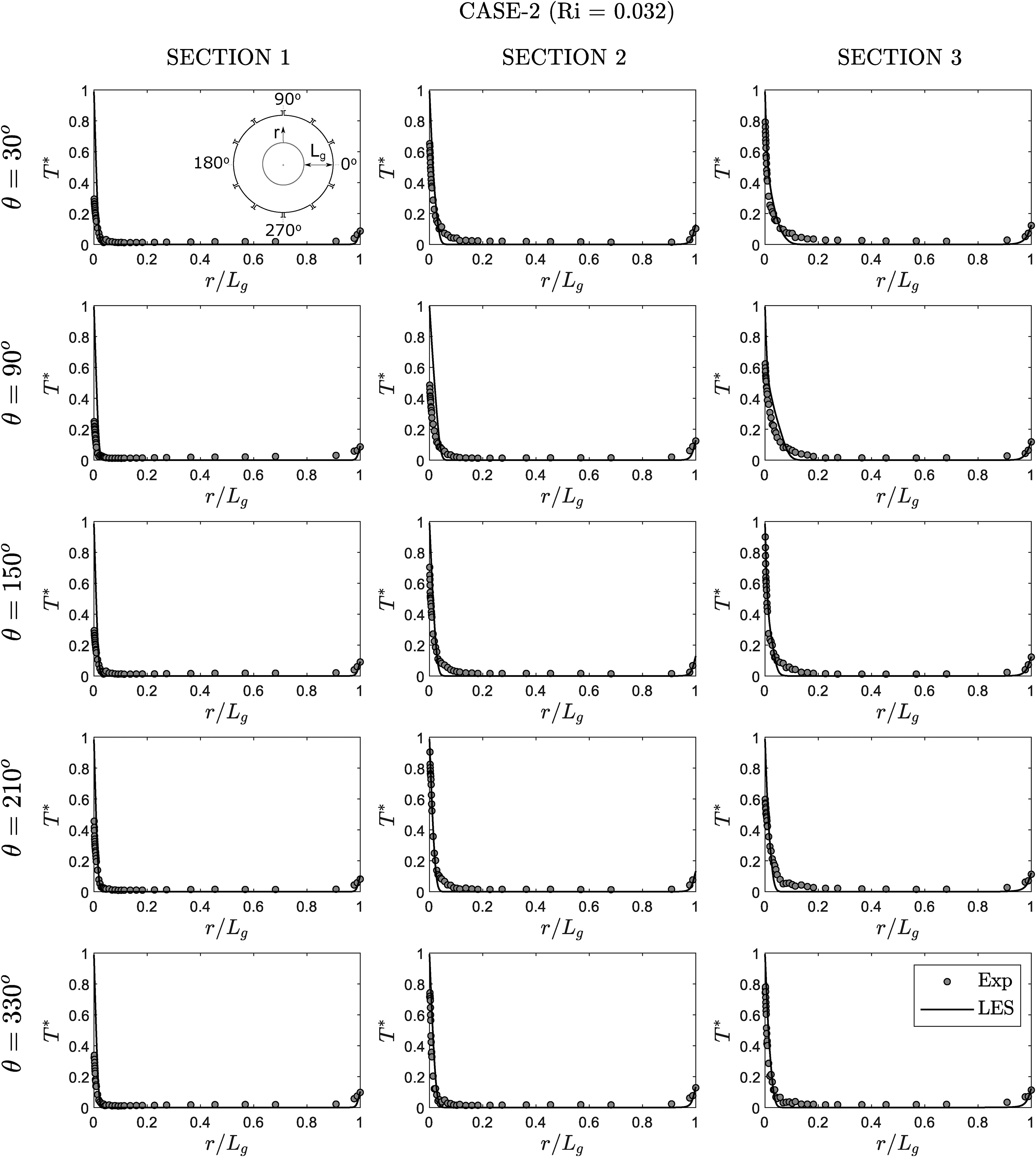
Figure 15 shows the temperature profiles from LES and the experiment for Case-2. As opposed to Case-1, Case-2 represents strong momentum of the fluid in the axial direction which reduces the effect of the buoyancy. At Section 1, there is a uniform temperature boundary layer around the inner cylinder which is well predicted by LES. At Section 2, the boundary layer is slightly thickened around the inner cylinder, however the temperature profiles at all measurement locations are very similar, which elucidates the dominance of the forced convection. This flow behaviour can also be seen in Figure 13 where there is no sign of clear plume development. At the upper portion of the annulus at Section 3, the temperature boundary boundary layer is slightly thicker than the lower portion. However, the thermal plume is still not present, therefore the temperature profiles in the annulus are not radically different . Overall, LES has exhibited a good agreement with the experimental data at all sections in Case-2.
Flow field
The flow field in the annulus can be investigated with the iso-surfaces and their footprints on the heated inner cylinder as illustrated in Figure 16 where the iso-surfaces of the second invariant of velocity
Figure 16.
(a) Iso-surfaces of second invariant of velocity, (b) Time-averaged wall shear stress around the inner cylinder.
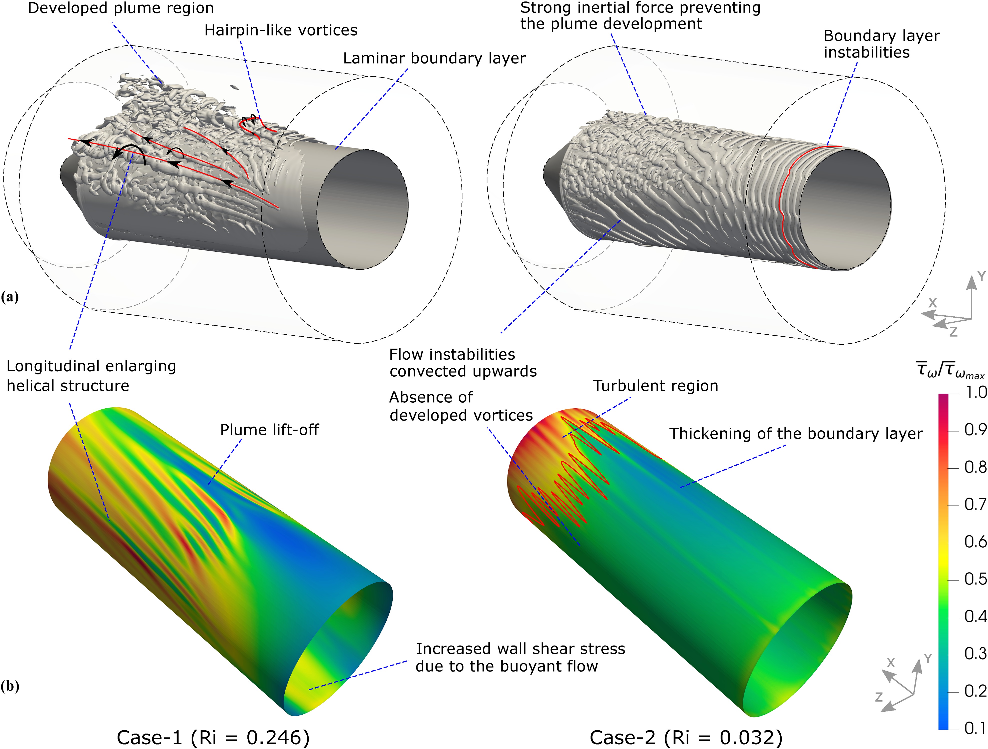
As opposed to Case-1 which represents a strong buoyancy influence in the flow field, Case-2 exhibits strong cross-flow influence which minimises the buoyancy effect. This phenomenon can be observed by looking at Case-2 iso-surfaces in 16a where the thermal plume is not formed at
Although the lower portion of the annulus remains laminar with both cases, there is a locally increased wall shear stress at the bottom of the inner cylinder in Case-1 due to the buoyant forces pushing the flow upwards against the inner cylinder which suppress the growth of the boundary layer. The shear stress distribution in Case-2 remains relatively uniform until the beginning of the turbulent region.
Heat transfer
Table 8 shows the detailed information on Nusselt number distribution at circumferential and axial measurement locations, which could be used for validation purposes. For Case-1, experimentally and numerically calculated Nusselt numbers as well as the LES errors are tabulated. Since the experimental heat transfer could not be obtained for Case-2 as described earlier, LES results are presented only for Case-2. Figure 17 illustrates the heat transfer distribution around the circumference at Sections 1–3.
Table 8.
Inner cylinder Nusselt number comparison.
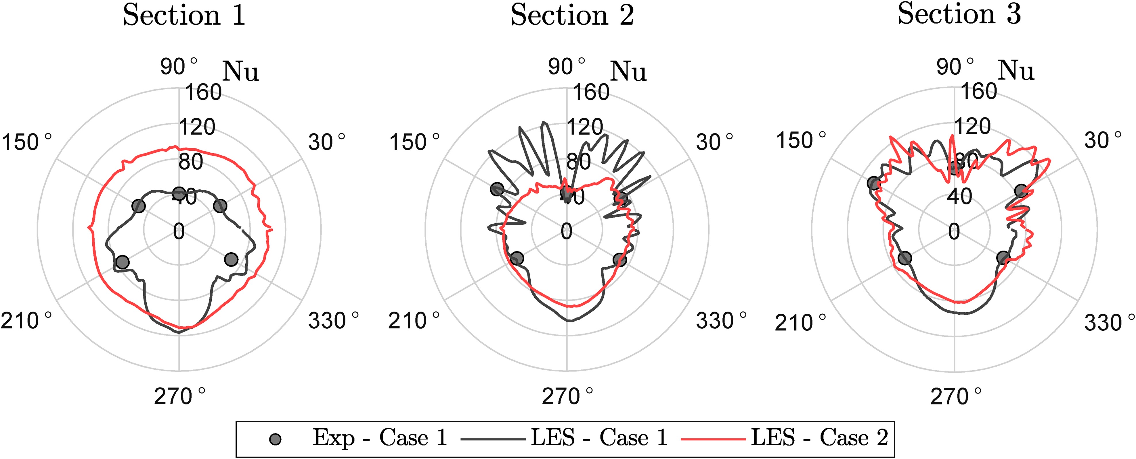
There is a heat transfer enhancement at the bottom of the inner cylinder compared to the top with Case-1, indicating that the buoyant flow causes a large temperature gradient (thin boundary layer) whereas Case-2 exhibits a uniform heat transfer around the inner cylinder at Section 1. The heat transfer drop phenomenon between the bottom and top in Case-1 is one of the well-known characteristics of the pure natural convection from a horizontal cylinder (Kenjereš and Hanjalić, 1995), which indicates the dominance of the natural convection. There are greater heat transfer values at each sides of the cylinder than that of the top. This could be attributed to the start of formation of the side helical structures. LES results show good agreement with Case-1 experiment with a maximum error of 21.95% at
At Section 2, the Nusselt number alternates remarkably at the upper half of the cylinder in Case-1 due to developed side structures, footprints of which are shown in Figure 16. Conversely, the bottom exhibits more uniform heat transfer rates which are slightly lower than Section 1 since the boundary layer is thicker. It is also interesting note that the minimum heat transfer has occurred at the top, indicating that the thermal plume lift-off has formed a large boundary layer. Although the highest LES error (-20.19%) has occurred at
Although there are still heat transfer minima/maxima at the upper half of the cylinder at Section 3 in Case-1, the fluctuations are not as strong as those at Section 2 since the flow is more developed at Section 3. Developing helical structures shown in Figure 16a have enhanced the heat transfer rates at both sides of the inner cylinder around
Conclusions
This paper has presented unique experimental data for mixed (natural and forced) type of flows which occur in turbine casing cavities during shut-down regimes. Detailed measurements have been performed in axial and circumferential directions to acquire detailed information in the large majority of the test section. Two experimental campaigns with different buoyancy force dominance have been performed to investigate the mixed convection cases at different rates since the real turbine casings are exposed to various mixed type of flows during shut-down regimes. Heat flux calculations from the thermocouple measurements have been discussed and the limitations due to the viscous sub-layer thickness have been highlighted. These experimental results can be used for the validation purposes and the development of the numerical tools for complex flow interactions in mixed type of flows. Additionally, large eddy simulations have been performed and validated against the experimental data. The scale resolving simulations have provided a great insight into the flow field with distinct flow structures for each case. In Case-1 where the buoyancy was more pronounced, a developed thermal plume region was observed towards the downstream with stretched helical structures at sides. The helical structures were found to cause large alternations in the heat transfer distribution around the inner cylinder. Case-2 where the dominance of the inertial forces was present exhibited almost circumferentially uniform boundary layer thickness. However, the varying enhanced heat transfer on the upper half of the heated inner cylinder was observed in the downstream due to the turbulent region.
These experimental and numerical results should contribute to the fundamental understanding of mixed type of flows in turbine casing cavities, which are of great importance for enabling flexible operations of the future power plants.
Nomenclature
Symbols
Bias error
Specific heat capacity (J/kgK)
Inner/Outer diameter (m)
Hydraulic diameter (
E
Error
f
Frequency (Hz)
Thermal conductivity (W/mK)
Gravitational acceleration (m/s2)
Heat transfer coefficient (W/m2K)
Grashof number
Gap width (m)
Nusselt number
Prandtl number
Radial direction
Goodness of the fit in linear regression
Reynolds number
Richardson number
Strain rate (1/s)
Time-averaged temperature (K)
Thermocouple bead temperature (K)
Effective surrounding temperature (K)
True fluid temperature (K)
Time-averaged wall shear stress (pascal)
U
Uncertainty
V
Variable
Second invariant of velocity (1/s2)
Vorticity magnitude (1/s)
Heat flux (W/m2)
Velocity (m/s)
Friction velocity (m/s)
Emissivity
Thermal expansion coefficient (1/K)
Kinematic viscosity (m2/s)
Angle (
Stephan-Boltzmann constant (5.6703×10⁸(W/m2K4))
Acronyms