Introduction

An aero-engine is a sophisticated aerothermodynamic mechanical system that undergoes performance degradation during its operation. Hence, effective and reliable monitoring and diagnosis of the engine is crucial to prevent mechanical failure and system collapse (Shen and Khorasani, 2020). Fault diagnosis and health management of the engine is highly dependent on the characteristics of its components, which are typically determined by engine manufacturers through costly testing and are not generally available to the public (Sun et al., 2020). Due to differences in test environments, test methods, and degradation of component characteristics during engine operation, there are often differences between component characteristics and test characteristics. Therefore, obtaining accurate component characteristics can be relatively difficult for engine users. Research on adaptation methods, such as modifying the characteristic maps or other component performance parameters in the component-level model to make the model prediction results consistent with the actual measurement results, is of great significant theoretical significance and engineering application value.

In recent years, there have been numerous studies aimed at correcting component performance maps or generating them directly from measured data. (Stamatis et al., 1990) introduced the concept of ‘modification factors’ to modify the performance maps of gas turbine performance models. (Lambiris et al., 1994) improved this method by incorporating adaptation calculations while solving for engine operating points. (Kong et al., 2003) proposed a method that uses scaling factors calculated from design points (DP) and component characteristics to improve the prediction of off-design performance. (Li et al., 2005; Li and Pilidis, 2010) have conducted extensive research in the area of performance model correction and proposed a scaling factor calculation method based on influence coefficient matrix (ICM) and genetic algorithm (GA). Furthermore, they proposed a method to modify the characteristic maps by fitting the speed and scaling factor for off-design points (Li et al., 2010, 2012). Alberto Misté and Benini (2014) introduced a method that directly adjusts the component characteristic map matrix instead of calculating the component correction factor and uses physical constraints on the characteristic map to limit the adjustment range. Tsoutsanis et al. (2012) introduced an elliptical curve as the compressor characteristic line and adjusted the component characteristic by manipulating the elliptical curve parameters using a genetic algorithm. Sun et al. (2021) represented the compressor characteristics as a Bezier curve and adjusted the Bezier curve control points using a genetic algorithm to match the model prediction parameters with the target gas path parameters.

Although many studies on engine performance adaptation methods have provided ways to correct the characteristics of engine components, they have mainly focused on situations where there is little variation in the working lines within a small operating range of the engine. However, no adaptation methods have been proposed for engines that operate over a wide range and cover multiple working lines. To address this issue, this paper presents a performance adaptation method for modifying aircraft engine characteristic maps over a wide operating range.

Methodology

Engine model

The research in this paper focuses on large bypass ratio turbofan engines. The established model mainly includes components such as the fan, booster, high-pressure compressor (HPC), high-pressure turbine (HPT), low-pressure turbine (LPT), and combustor, as shown in Figure 1, where the numbers indicate the station positions.

Figure 1.

Model engine configuration.

Characteristic maps adaptation method

During engine model calculations, the component characteristics are stored in a computer in tabular form. By interpolating the component corrected mass flow, pressure ratio, and efficiency in the two-dimensional table using the relative corrected speed Ncr and the auxiliary value Beta, the characteristics of the components are obtained. When there is a difference between the real characteristic map and the original characteristic map, the characteristics obtained from the characteristics table under the same working conditions will be different, which ultimately causes a deviation between the model prediction and the real measurement.

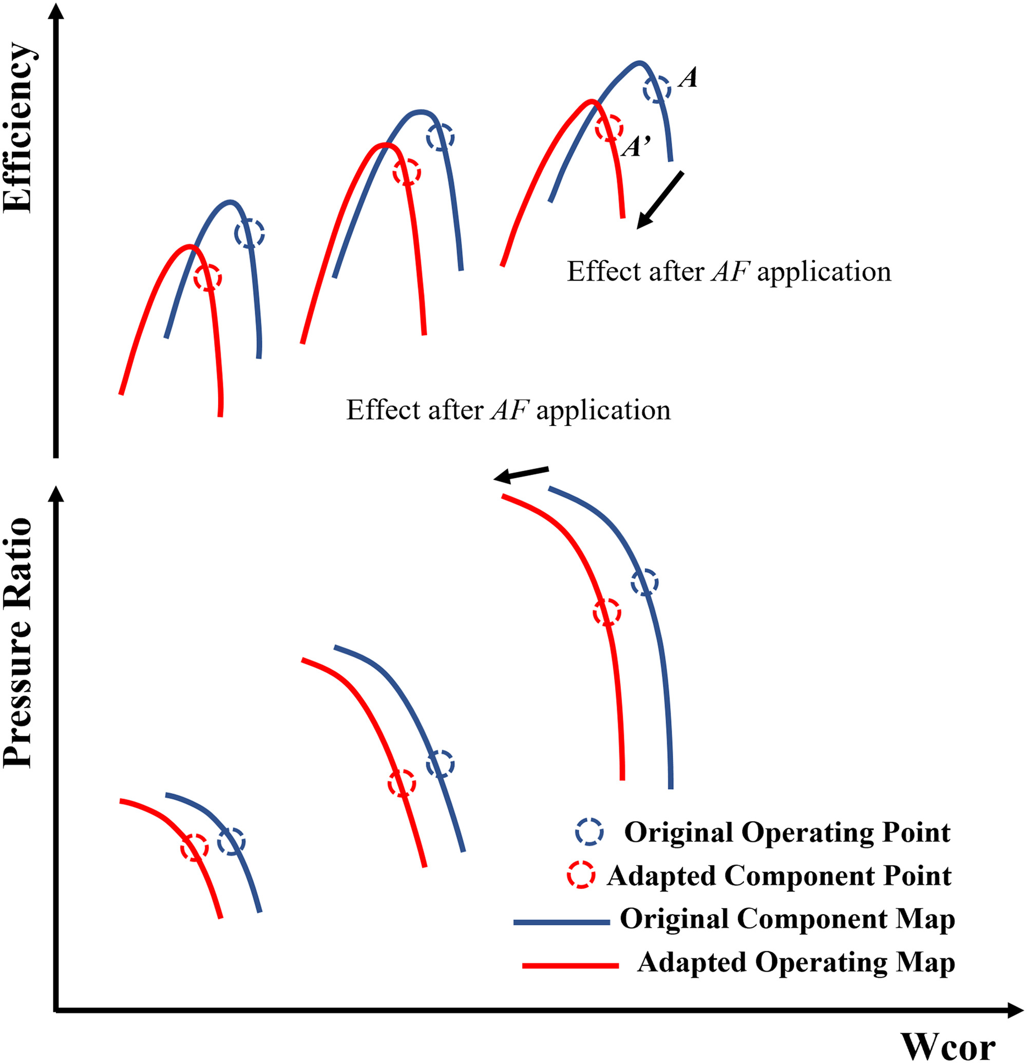
To correct the deviation between the model prediction and the measurement, the adaptation factor is introduced into the component calculation to adjust the original characteristic map. Taking the fan as an example, the mass flow and efficiency adaptation factors are defined as Equations 1 and 2, where Wcor_A′ and ETA_A′ are the corrected mass flow and efficiency of the real engine under this operating condition, Wcor_A and ETA_A are the corrected mass flow and efficiency read from the original characteristic map when the model prediction matches the measurement. The effect of the adaptation factor is shown in Figure 2, which can stretch and shift the map to make it closer to the real characteristic map.

Figure 2.

Adaptation of compressor map.

(1)

AFW=WcorA′WcorA.

(2)

AFE=ETAA′ETAA.

This study focuses on the analysis of an engine consisting of five primary rotating components, namely FAN, Booster, HPC, HPT, LPT. Each component is characterized by two adaptation factors, as demonstrated in Table 1. In total, the model incorporates 10 adaptation factors.

Table 1.

Adaptation factors for components.

Component	Mass flow adaptation factor	Efficiency adaptation factor
FAN	AFWFAN	AFEFAN
Booster	AFWBooster	AFEBooster
HPC	AFWHPC	AFEHPC
HPT	AFWHPT	AFEHPT
LPT	AFWLPT	AFELPT

Solving for the adaptation factor

The method used to solve the adaptation factor for each operating point is the Newton-Raphson method. The iterative calculation formula is given by Equation 3, where J is the Jacobian matrix, x is the variable for the iterative calculation, and ek is the residual of the target (Li et al., 2021).

(3)

xk+1=xk−J−1ek.

After introducing the adaptation factors, the engine model must not only satisfy the balance equation, but also ensure that the residual between the model prediction and the measurement is less than 1 × 10⁻³.

The Newton-Raphson method is known for its fast convergence and high accuracy in local convergence during computation. However, it is also sensitive to the original trial values, which can lead to oscillations and divergences, especially when correcting characteristic maps, as investigated in this paper. To address these problems associated with the Newton-Raphson method, this paper proposes a hybrid algorithm to improve the convergence of correction factor calculations. This algorithm combines the Newton-Raphson method with global optimization algorithms for the calculations.

Particle Swarm Optimization (PSO) (Kennedy and Eberhart, 1995) is a heuristic algorithm commonly used to solve optimization problems by simulating the information sharing and cooperative behaviour of individuals in a population. Each individual is represented as a particle in the search space and explores it by adjusting its position and velocity. The algorithm evaluates the fitness of each particle by measuring the objective function and updates its velocity and position by sharing information with other particles in each iteration. The PSO algorithm is known for its global search capability, simplicity, ease of use, and parallelizability, making it a popular choice in many fields. In this paper, PSO is used to perform global search for adaptation factors.

The main steps of PSO include initialization, velocity update, position update, fitness evaluation, and global best update. PSO requires setting appropriate parameters and defining a fitness function to evaluate individuals, i.e., the degree of adaptation of the optimal solution to the problem. The parameters of PSO are set as follows: maximum generation of 300, population size of 50, velocity inertia weight of 0.8, self-learning factor of 1.5, and group learning factor of 1.5. The fitness function defined in this paper is Equation 4 as follows: where P_model represents the model calculation result, P_real represents the measurements, and σi represents the weights, all set to 1.

(4)

OF=∑1mσi|(Pmodel−Preal)|/Preal.

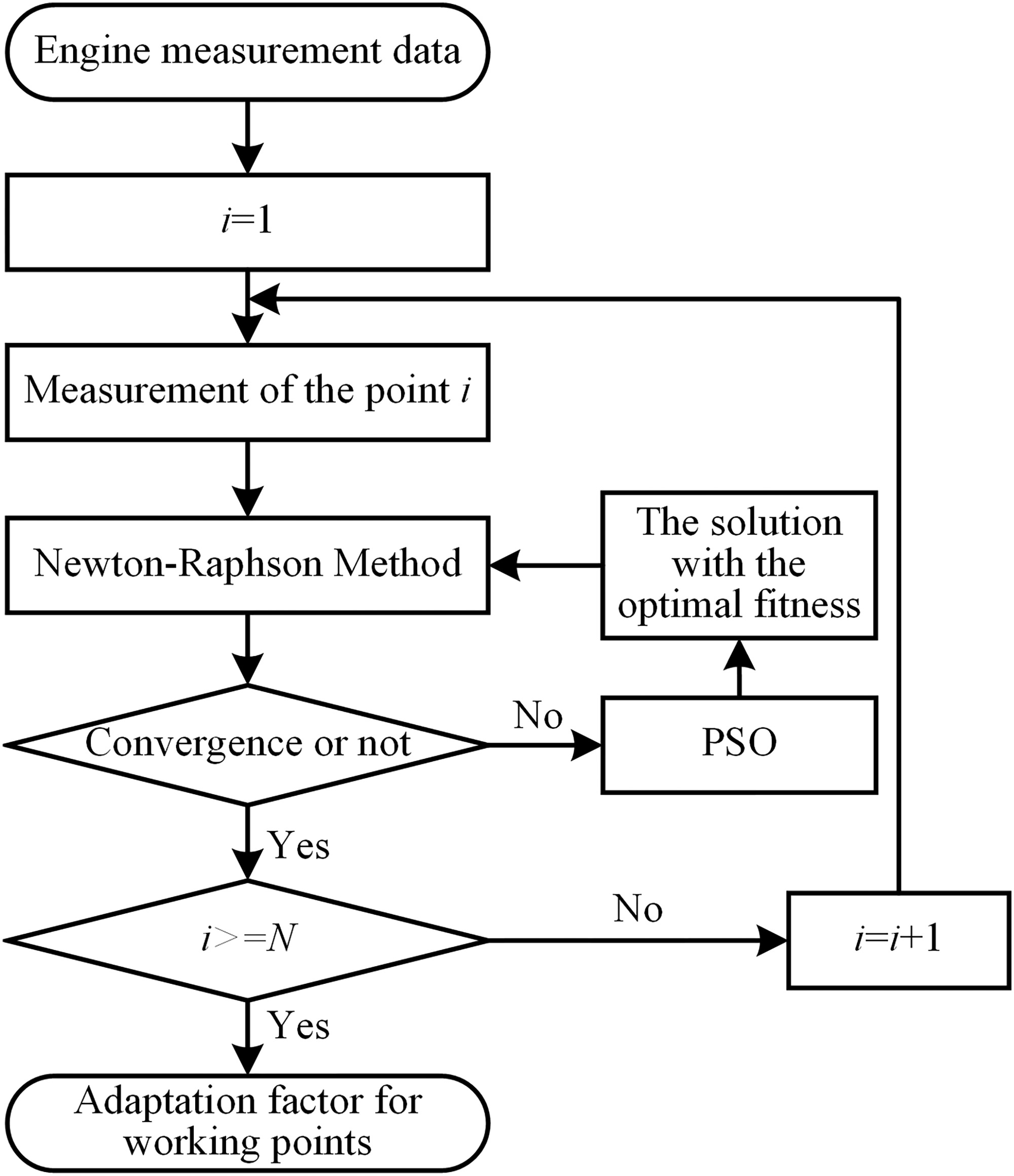
Specifically, for each operating point, the calculation is first attempted using the Newton-Raphson method. If the method fails to converge, the calculation is then performed using PSO. The initial population generated by PSO contains the trial value with the optimal fitness from the iteration of the Newton-Raphson algorithm. The optimal solution obtained by PSO is then substituted into the Newton-Raphson method for recalculation until convergence is reached. The detailed calculation process is shown in the Figure 3.

Figure 3.

Hybrid algorithm flow for solving the adaptation factor.

Adaptation factor surface

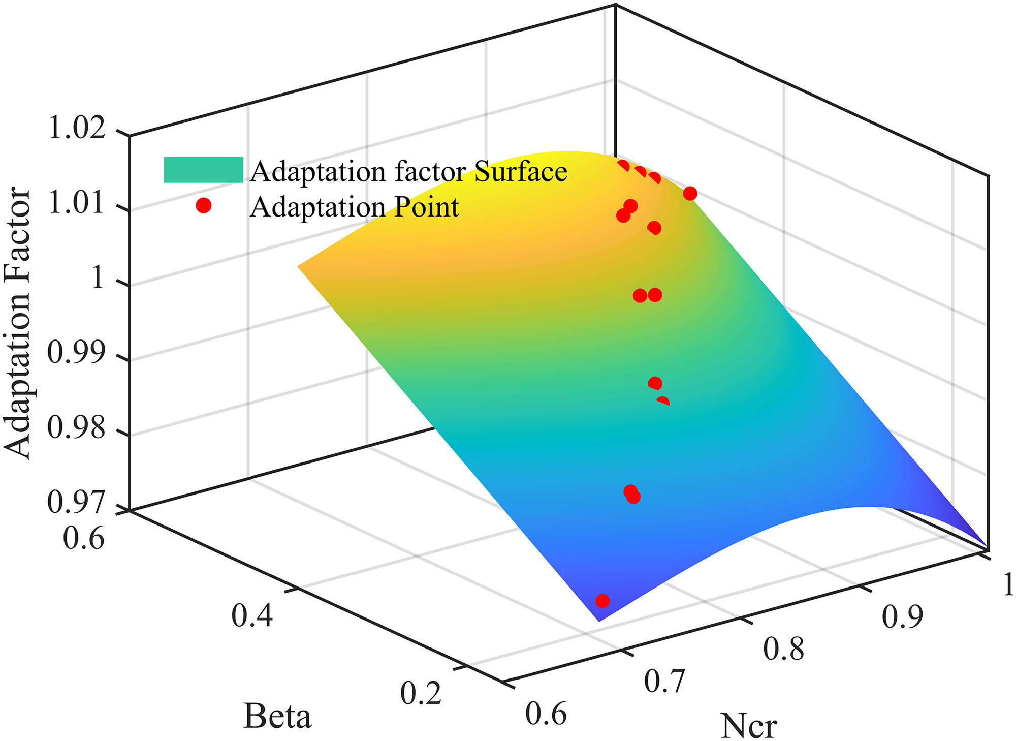
Traditionally, the adaptation method assumes that the adaptation factor changes with speed, and this relationship can be represented as a function with speed as the independent variable and the adaptation factor as the dependent variable. This method is referred to as the adaptation factor curve method in this paper. However, it has an inherent limitation - it cannot personalize the correction of points on the equal speed line. To overcome this limitation, this paper proposes a novel multi-point map matching method for engine performance correction using the adaptation factor surface. The method establishes a correlation between the adaptation factor and the relative corrected speed and characteristic map Beta, thus allowing the characteristic map to be adjusted in two directions. When the adaptation factor is drawn with the relative corrected speed as the x-axis and beta as the y-axis, the resulting curve is a surface as shown in Figure 4. Therefore, by solving the functional relationship of the adaptation factor surface, the method can make more accurate corrections to the working points on the characteristic map, ensuring that the corrected characteristic map approximates the real characteristic map in both the relative corrected speed and beta dimensions.

Figure 4.

Adaptation factor Surface.

By means of least squares, the functional relationship of the adaptation factor surface can be obtained, assuming that it takes the form of Equation 5

(5)

AF=p1+p2f1(Ncr,β)+p3f3(Ncr,β)+…+pnfn(Ncr,β).

where and are known functions of the relative corrected speed and Beta, respectively, and is a constant coefficient to be solved. In this study, it is hypothesized that the functional relationship of the adaptation factor surface can be expressed as Equation 6.

(6)

AF=p1+p2Ncr+p3β+p4Ncr2+p5Ncr3.

Results and discussion

In order to evaluate the developed multi-point adaptation method, the large bypass-ratio turbofan engine model described in the previous section was used. Two sets of characteristic maps were used - one as the characteristic map of the original uncorrected model, and the other as the “real characteristic map” that generated measured data for a real engine. The measurement parameters used for the adaptation computation are detailed in the Table 2.

In this case study, a subset of operating points was identified as adaptation points, while another subset of steady-state points were identified as test points to evaluate the effectiveness of the developed method. A comprehensive list of the adaptation and test points, along with the relative corrected speed and beta values of the fan component, is presented in Table 3.

Figure 5 illustrates the placement of the adaptation and test points on the original fan map. It is evident that these operating points are distributed over several regions of the fan map rather than along a single operating line.

Figure 5.

Location of the adaptation and test points in the FAN map.

At each working point, we calculated the adaptation factors AFW and AFE and fitted 10 adaptation factor surface functions for the 5 components. Then, we incorporated these adaptation factor surface functions into the model to improve the prediction accuracy and reduce the error between the prediction and measurement.

The effectiveness of the adaptation factor surface method in reducing model errors was evaluated by correcting the original model using two methods: the adaptation factor surface method and the adaptation factor curve method. The corrected model was then used to calculate predicted parameters at seven adaptation points and seven test points. The prediction errors of each parameter were created, as shown in Figure 6, and a table was generated to compare the performance of the model before and after the adaptation corrections. For example, the original model had significant errors between the predicted and measured values of WF, with the errors increasing as the measured values of WF increased. The maximum error exceeded 25%. However, after the model was corrected using the adaptation factor curves, the errors were significantly reduced, especially at operating points with higher WF. After correcting the original model using the adaptation factor surface method, the error between the predicted and measured values decreased significantly, and the working points aligned almost perfectly with the diagonal line representing “Error = 0” on the error graph.

Figure 6.

Prediction error for each parameter.

Observation of Figure 6 reveals that that out of all the measured parameters, P13 had the smallest model calibration error. For those parameters with comparatively small original errors, the calibrated errors after correction remained relatively small when compared to other parameters. On the other hand, for those parameters with larger original errors, the calibrated errors after correction remained relatively larger compared to other parameters, such as WF and P45.

A three-dimensional scatter plot of the parameter prediction errors was generated to investigate the relationship between the adaptation effects and the operating point position, as shown in Figure 7. The x-axis represents the relative corrected speed of the fan component, the y-axis represents the Beta value of the fan component characteristic curve, and the z-axis represents the prediction error of each parameter. The results show that the errors of the measured parameters were higher when moving away from the design point, and the errors increased as the relative corrected speed decreased. However, no clear trend was observed in the beta direction.

Figure 7.

Three-dimensional scatter distribution of the prediction error of the parameters.

Table 4 presents a summary of the mean prediction errors for all parameters before and after the adaptation of performance models across 14 operating points. The adaptation methods employed were the adaptation factor curve method and the adaptation factor surface method. Prior to adaptation, the mean error between model prediction and measurement was significantly large, exceeding 40% and even exceeding two times for the maximum mean error. However, the introduction of the adaptation factor curve correction resulted in a reduction of over 50% in the mean deviation of ten measurement parameters, resulting in an overall mean error reduction of 20.423%. Nevertheless, certain parameters, such as WF, P25, P3, and P45, still showed large mean deviations of more than 30% even after the correction. This suggests that the adaptation factor curve method struggled to achieve optimal expected correction effects in the current case. Conversely, the surface method was able to reduce the mean deviation of all parameters to a negligible level, with all parameters showing deviations below 1% and an overall mean deviation of only 0.29%. These results suggest that the adaptation factor surface method can achieve the ideal prediction error target even when the operating points are widely dispersed.

Figures 8, 9 and 10 show a comparison between the original characteristics, the real characteristics, and the characteristics corrected by the adaptation factor surface method of Booster, HPC, and LPT. The original, real, and corrected working points of the components are also shown. Before the adaptation correction, there was a significant deviation between the original characteristic line and the real characteristic line. The adaptation correction caused the original characteristic line to stretch, bend and shift to a new position. As a result, the corrected curve is closer to the real curve in the region covered by the working points. In addition, it is observed that the original working point and the real working point are quite far apart, while the corrected working point almost coincides with the real working point, indicating a high degree of similarity between the working performance of the model component and the real component. It is worth noting that the characteristic line after the correction shows a bending change. This effect is intentional, as the range of the adaptation factor was limited during the correction process to avoid the occurrence of an inappropriate adaptation factor surface.

Figure 8.

Original, real and adapted characteristics of Booster.

Figure 9.

Original, real and adapted characteristics of HPC.

Figure 10.

Original, real and adapted characteristics of LPT.

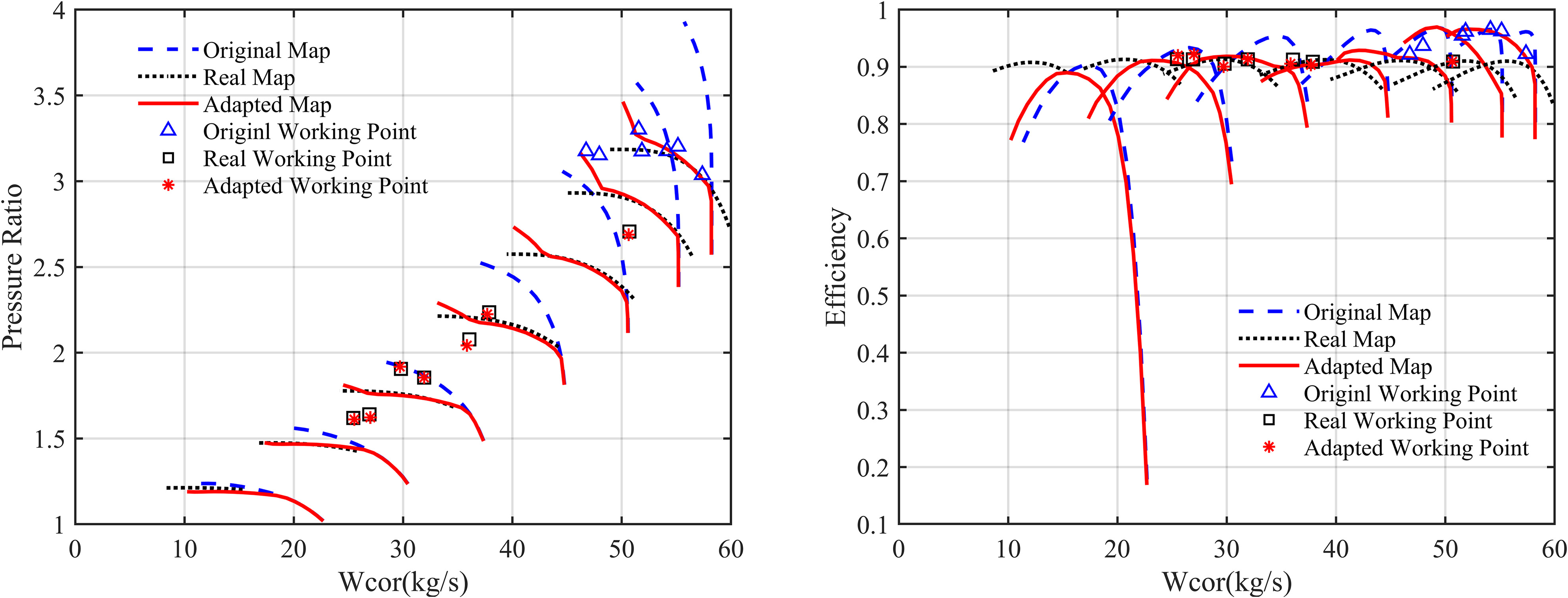
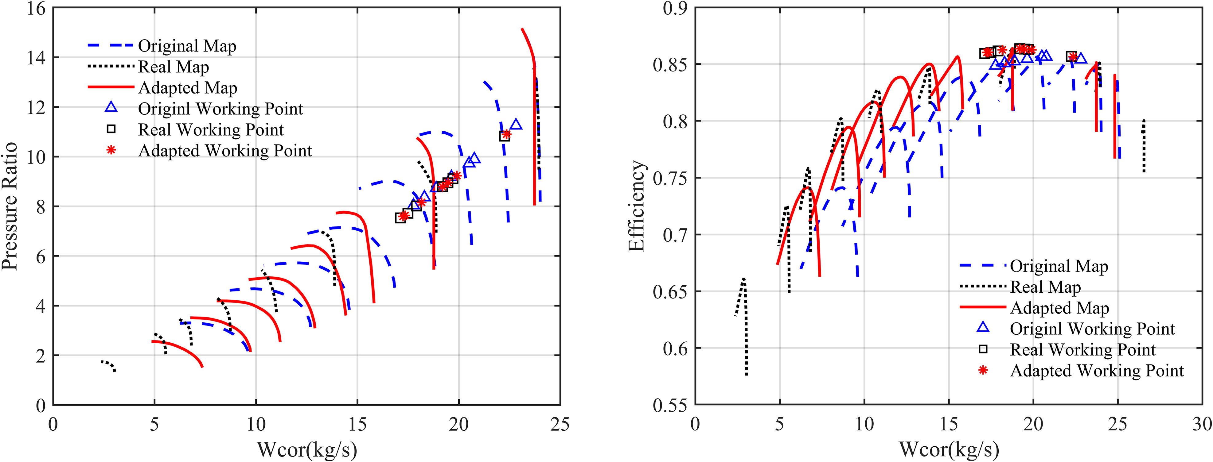
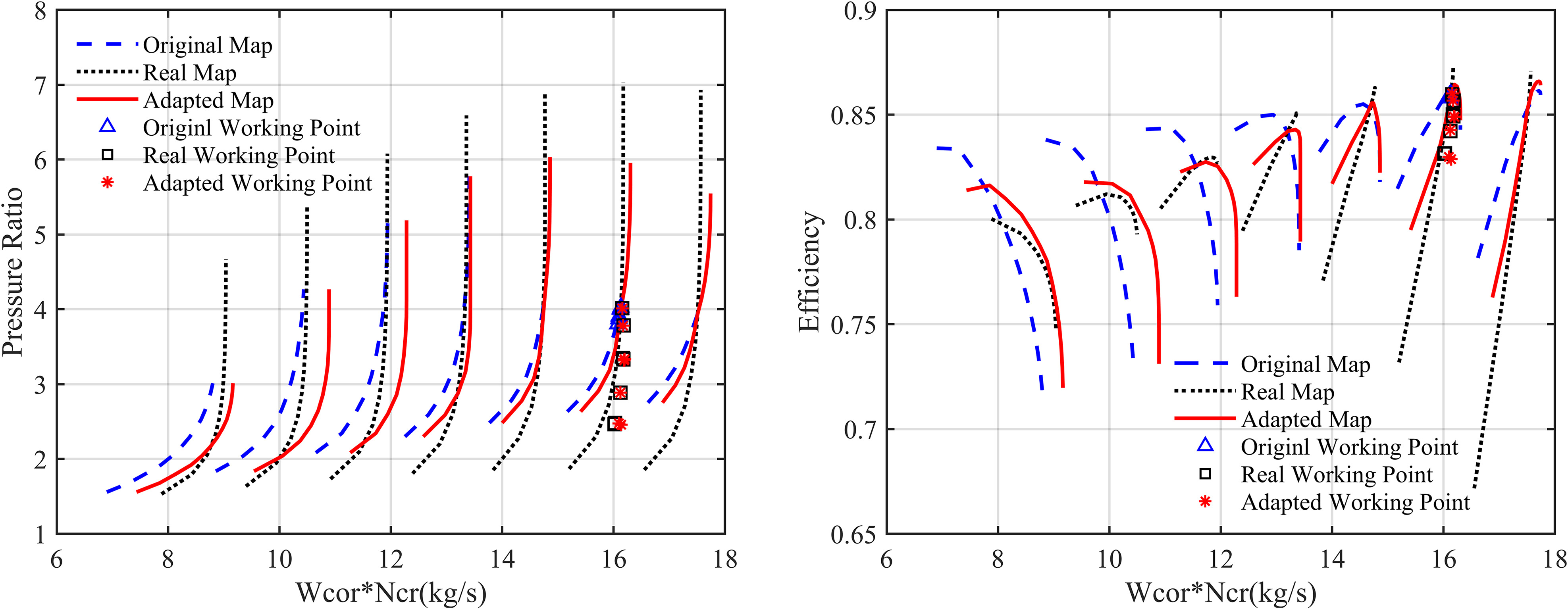
Figure 10 compares the original, real and corrected performance maps of the LPT and plots the original, real and corrected working points of the components. It is noteworthy that the turbine components behave differently than the compressor components, with the working point of the turbine components showing relatively little movement with changes in operating conditions. Consequently, the corrected performance maps of the turbine components show smaller changes compared to those of the compressor components.

Conclusions

This paper presents a performance adaptation scheme for aircraft engines over a wide operating range. The scheme introduces the difference between the component performance of the adaptation factor representation model and the real engine, and it provides a mixed solution algorithm for calculating the adaptation factor of the operating points, which combines the advantages of the Newton-Raphson method and the global optimization algorithm. The correlation between the relative corrected speed, beta value and the adaptation factor is then established to fit the adaptation factor surface and achieve the correction and adjustment of the characteristic map in the two directions of relative corrected speed and beta value.

To verify the effectiveness of the proposed scheme, case studies are designed, and the results show that:

Nomenclature