
Introduction
Numerical zooming is a computational approach used in aero engine design and analysis to study the flow characteristics in specific regions of interest within the engine (Jia et al., 2022; Xu et al., 2022; Yang et al., 2022; Zheng et al., 2023). The Cycle with CFD in it (CWCFD) method in numerical zooming involves integrating multiple models with varying fidelity and complexity into a full engine simulation. This approach is particularly useful in regions of high aerodynamic loading, such as compressor and turbine, where the flow is complex and can significantly affect engine performance (Pachidis et al., 2006, 2007a, 2007b; Klein et al., 2017; Briones et al., 2021). By coupling 3D CFD models of these regions, the CWCFD method can obtain more accurate information and better understand the impact of design changes on engine performance. Overall, the CWCFD method in numerical zooming is powerful in aeroengine design and analysis, allowing for a more comprehensive understanding of the complex flow characteristics occurring within the engine (Lytle, 2006; Schlu Ter et al., 2006; Bala, 2007; Medic et al., 2007; Pachidis et al., 2007a).
The component-level models (CLM) are conventionally used in simulating the overall performance of gas turbines due to their fast computational speed and simple implementation. However, their precision is primarily dependent on characteristic maps and falls short in capturing detailed information about components (Zhou et al., 2019; Pang et al., 2020; Jia et al., 2021; Hao et al., 2022; Wang et al., 2023; Zhuang et al., 2023). To incorporate high fidelity into the component-level model and eliminate the reliance on characteristic maps, the CWCFD zooming method has emerged as an extensively researched avenue.
The CWCFD zooming method directly embeds the CFD models into the CLM cycle. Research on the CWCFD method embedding the 1D inlet and nozzle CFD models was first conducted. Connolly utilized this approach to investigate the dynamic response of engine thrust (Connolly et al., 2014), while Allison analyzed the impact of different attack angles on engine installation performance at supersonic speeds by embedding a 1D intake model into the entire engine CLM cycle (Allison and Alyanak, 2014). In summary, these efforts yielded improvements in simulation accuracy and the capture of detailed flow fields. However, it's worth noting that the application of CWCFD zooming methods has predominantly focused on non-rotating components, with limited attention to the high-fidelity integration of rotating components.
Unfortunately, embedding 3D CFD rotating component models in the CWCFD zooming method presents a significant challenge due to convergence issues. To address this, Fu incorporated a high-fidelity model of a non-rotating component into the CLM of a variable cycle engine model (Song et al., 2021), while Pilet added an interface between mass flow and static pressure to integrate the CWCFD zooming method into a CLM with only the 3D CFD model of a rotating fan (Pilet et al., 2011). Despite these endeavors, the incorporation of multiple 3D CFD rotating component models, such as those of compressors and turbines, remains a formidable challenge. Simulations often focus on the design point or a few off-design points near it and typically involve the coupling of a single rotating component. Consequently, extending the applicability of CWCFD zooming methods to encompass multiple rotating components and broader operational ranges in complex engines poses a significant challenge.
To address these challenges, the present study proposes a CWCFD zooming method coupled compressor and turbine with high fidelity. The proposed CWCFD zooming method is implemented by embedding the multiple 3D CFD models of compressor and turbine (coaxial rotating), rather than the corresponding characteristic maps, into the CLM cycle of a gas turbine. The method is used to simulate the overall performance of a KJ66 gas turbine over a wide range of off-design points. The method is compared with the traditional CLM method, and the experimental data of a ground test is used to verify its effectiveness. Overall, its application to the industry seems to be promising. The proposed method allows us to know more detailed information about flow characteristics in an engine, improving the accuracy of data, without using characteristic maps.
Methodology
Research objects
The KJ66 micro gas turbine (MGT) has gained a reputation as a mature commercial engine, with publicly available data. Its dimensions are noteworthy, with a diameter of around 110 mm, a length of about 240 mm, and a total weight of approximately 0.93 kg. This engine can produce a maximum thrust of 84.5 N, and it consists of three key components: a centrifugal compressor, an axial turbine, and a burner. The engine has been the subject of numerous studies on its components and overall performance, with several researchers dedicating time to investigate (Xiang et al., 2017; Xu et al., 2022; Yang et al., 2022). Additionally, experimental data on thrust, rotational speed, and specific fuel consumption is available in Ref. (Schreckling, 2005) and will be used for comparative analysis in the next section of the paper. It is noteworthy that all of these performance metrics were obtained under sea-level conditions based on the International Standard Atmosphere (ISA). Table 1 presents a comprehensive list of the design parameters and performance characteristics of the KJ66 MGT.
Table 1.
Design parameters and performance characteristics of the KJ66 MGT.
Component-level model
The component-level model (CLM) is a simulation approach for aeroengines that does not involve the use of computational fluid dynamics (CFD). Instead, it relies on a set of equations and algorithms to represent the performance of each component within the engine. The model breaks down the engine into its main components, such as the compressor, turbine, and combustion chamber, and simulates each component's behavior based on its operating conditions and performance characteristics. The model uses a combination of theoretical equations, empirical data, and experimental results to predict the overall performance of the engine. The component-level model allows for a rapid evaluation of the engine's performance under various operating conditions and can aid in optimizing engine design and operation.
In this paper, the authors have developed a CLM that is derived from the fundamental principles of conservation of mass flow, pressure balance, and power balance. These equations are used to establish the cooperation equations that represent the relationships between the various components of the engine. The CLM focuses on simulating the behavior of the compressor and turbine, which are critical components of the engine. The corresponding cooperation equations of CLM are established, including the relative error of the compressor and turbine mass flow, turbine and exhaust mass flow, and compressor and turbine power in the cooperation equations.
First, the conservation of mass flow between compressor and turbine without consideration of air bleed:
Second, the conservation of mass flow between the turbine and exhaust:Third, the power balance between compressor and turbine without consideration of power extraction:
The CLM relies on the characteristic maps of the compressor and turbine, which are typically obtained through extensive experimental testing or numerical simulation. These maps describe the behavior of the components as a function of various operating parameters, such as rotational speed and pressure ratio. In the CLM model, these maps are used to calculate the mass flow and power of the components, which are then used to determine the overall performance of the engine. The characteristic maps are expressed as Equation 4 and include parameters where
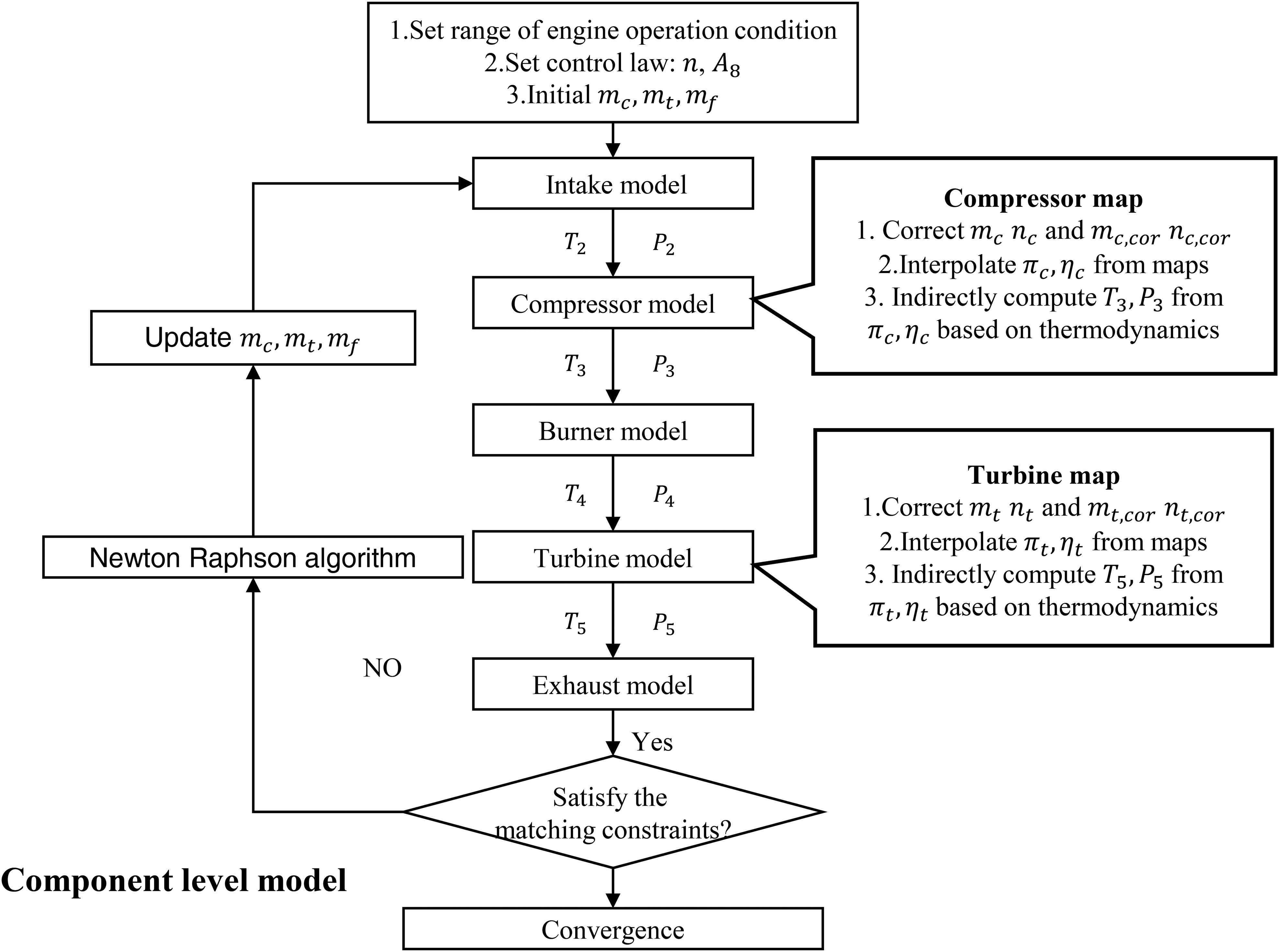
The flowchart of the CLM for KJ66 MGT is depicted in Figure 1, which consists of six distinct modules. The first module is the intake model, which calculates the intake thermodynamic parameters based on the given flight conditions. The compressor and turbine modules, on the other hand, interpolate the component characteristic parameters using the characteristic maps and calculate thermodynamic parameters. The burner module determines the burner characteristics through empirical expressions, while the exhaust module computes thermodynamic parameters based on the state of the exhaust. Finally, the Newton-Raphson solver uses an iterative approach to solve the cooperation equations.
3D CFD models of rotating components
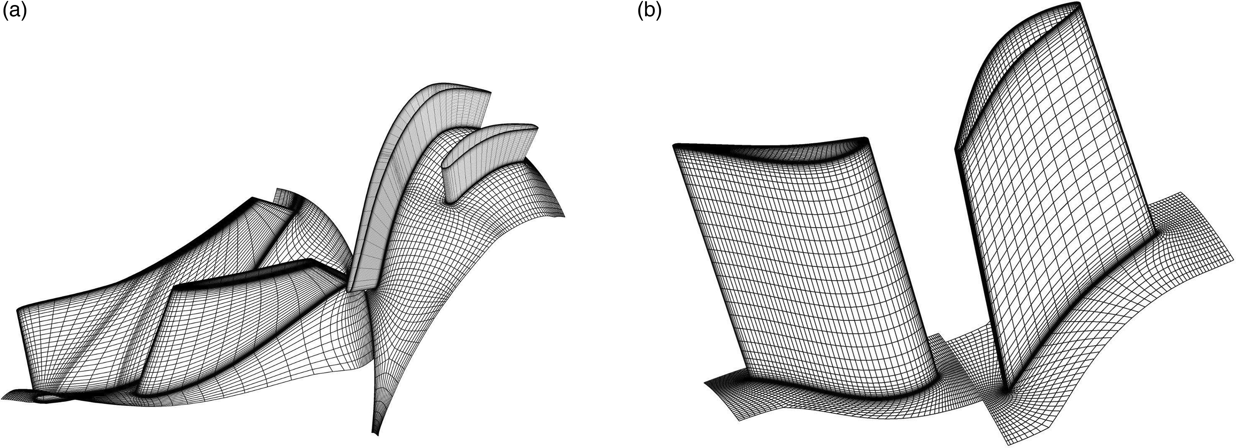
The 3D CFD models of the compressor and turbine in the CWCFD zooming method were utilized through ANSYS CFX. To verify the reliability of the 3D simulation results, Table 2 presents various grid configurations (serial numbers 1–3) along with the corresponding grid numbers for the 3D models. Notably, the selected mesh number per blade passage of both the impellor and diffuser was approximately 700,000, and the selected mesh number per blade passage of both the vane and rotor was approximately 750,000. This indicates that the characteristic parameters of these components did not change significantly with increasing mesh count. To reduce computational costs, a single-blade passage was used for the impellor, diffuser, turbine vane, and rotor. Further information about the chosen 3D meshes for the compressor and turbine CFD models can be seen in Figure 2.
Table 2.
Various grid configurations of component.
Figure 2.
3D meshes for the compressor and turbine CFD models. (a) Compressor mesh. (b) Turbine mesh.
The steady RANS equations were solved using a finite control volume method. A mixing plane approach was employed as the rotor-stator interface of the computational domain. To model turbulence, the k-ε turbulent model with scalable wall functions was used according to the previous verification (Briones et al., 2020, 2021). The y-plus near the wall met the requirement for calculating the boundary velocity with scalable wall functions. The inlet boundary of the compressor and turbine was the flow direction, total pressure, and total temperature, and the outlet boundary was the mass flow. The rotational speed was also input to CFD models. After these, the 3D steady numerical simulation of the above two components is solved.
In addition, the total outlet temperature and pressure of the compressor and turbine are obtained directly from the averaged mass flow using CFD models. In addition, the power of the compressor and turbine is obtained directly by numerical integration using CFD models. This differs significantly from the component-level model, where the total outlet temperature, pressure, and power of the compressor and turbine are calculated indirectly from the efficiency and pressure ratio according to the thermodynamic principle. In summary, the high-fidelity model of the compressor and turbine can be expressed as Equations 5 and 6.
where L is the torque of the rotating parts of the compressor or turbine, S is the surface comprising all rotating parts,
CWCFD zooming method
In the original cooperation equations of KJ66 MGT, the components had three independent variables. However, by replacing the characteristic maps with those obtained from 3D CFD models, it became possible to choose the independent variables of the cooperation equations as real mass flow directly instead of the corrected mass flow. This allowed for a direct exchange of parameters between the CLM and CFD models without any transformation. Therefore, in the modified cooperation equations, as shown in Equation 7, the mass flow of the compressor
For simplicity, the cooperation equations can be expressed as
The Newton-Raphson method iteratively solves the cooperation equations until the accuracy standard
In summary, the CWCFD zooming method eliminates the need for characteristic maps and the correction between actual conditions and ISA. This means that the corrected mass flow and rotational speed are not required, and the compressor and turbine characteristics can be expressed directly. In contrast, the CLM method indirectly computes the outlet total temperature and pressure of the compressor and turbine from efficiency and pressure ratio according to thermodynamics.
The schematic of the CWCFD zooming model built for KJ66 in this paper is shown in Figure 3, which realizes the zooming of the dual rotating components, including the compressor and turbine. The 0D components model of the intake, burner, and exhaust are built by SIMULINK/MATLAB, which are the same in the CWCFD zooming model and the CLM. The component characteristic parameters of the compressor and turbine are obtained by self-programmed CFX macro scripts. The 3D CFD models of the compressor and turbine are directly embedded in the corresponding engine SIMULINK module using self-programmed Python communication scripts, which is significantly different from the interpolation-based 0D component module of the compressor and turbine in CLM. The Newton-Raphson solver iteratively solves the cooperation equations until the error criteria are satisfied.
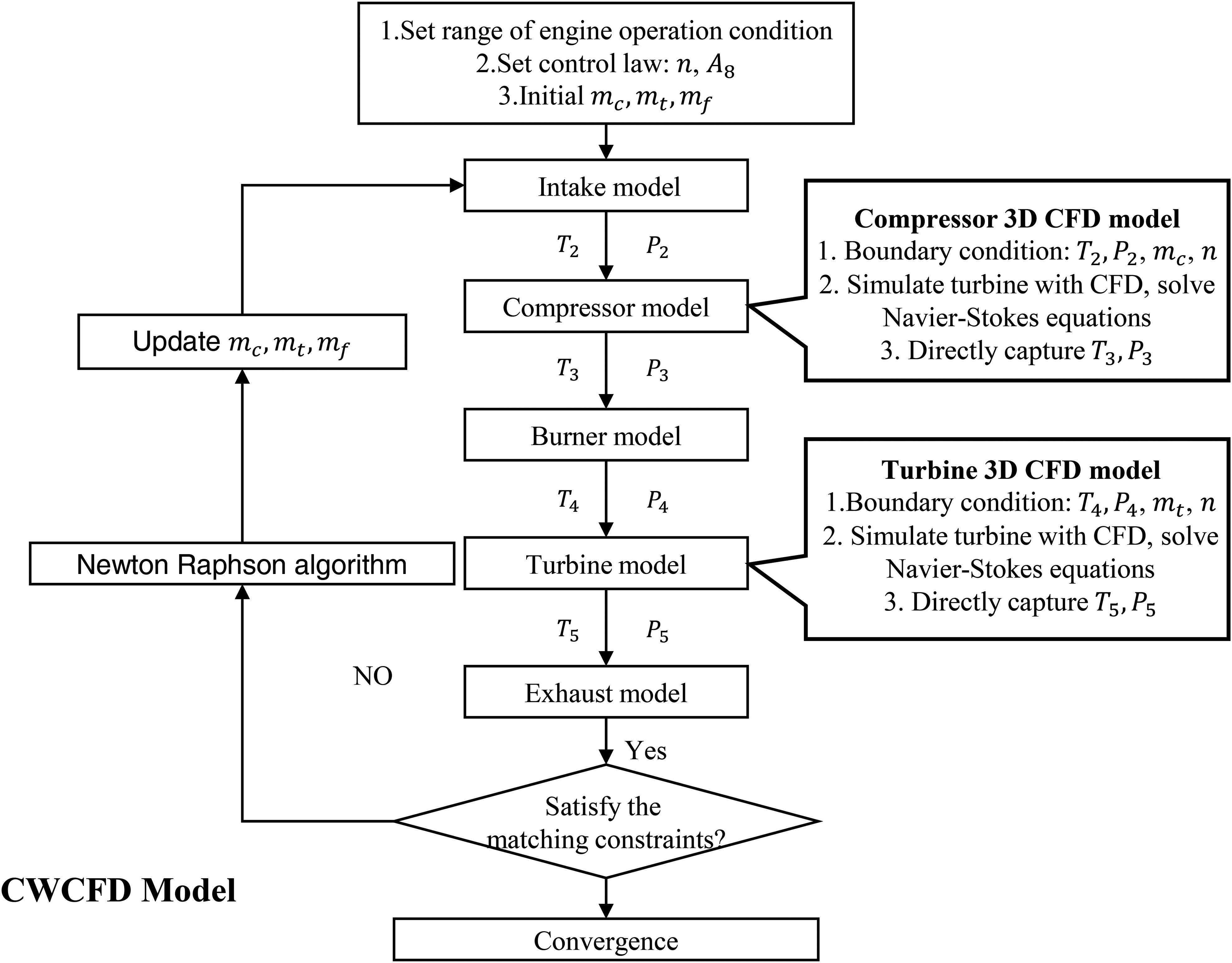
The CWCFD zooming model used in this study comprises three main modules, namely, 0D component modules, 3D CFD models, and a cycle-solving module. The 0D component modules calculate the characteristics of non-rotating components such as the intake, burner, and exhaust using existing empirical correlations. On the other hand, the 3D CFD models are used to simulate and extract the characteristic parameters of the compressor and turbine. To transfer the parameters from the 0D component module to the corresponding boundary conditions of the 3D CFD model, a uniform distribution is used, including the compressor and turbine total inlet temperature, and total inlet pressure. Furthermore, the 3D distribution of interface parameters simulated by the 3D CFD model is directly transferred to the 0D thermodynamic parameters through mass flow averaging. The 0D component module and the 3D CFD model are run sequentially according to the physical assembly sequence. The cycle solving module calculates the errors and then iteratively solves the cooperation equations using the Newton-Raphson method until the error criteria are satisfied.
Results and discussion
The effectiveness of the CWCFD zooming method was evaluated by simulating the throttle characteristics of the KJ66 MGT at a wide range of off-design conditions. To achieve the throttle characteristics at ISA, several rotational speeds ranging from 60,000 to 120,000 RPM were selected to calculate the thrust, specific fuel consumption
To quantify the error between the numerical simulation results and the experimental data, the global error
Figure 4 presents a comparative analysis of the experimental and numerical simulation results obtained through the CWCFD and CLM methods. The results indicate that both methods demonstrate a high level of prediction accuracy for parameters, thrust, and
Figure 4.
Comparison of throttle characteristics of KJ66 MGT. (a) Thrust. (b) Compressor outlet total temperature. (c) Turbine outlet total temperature. (d) Specific fuel consumption.
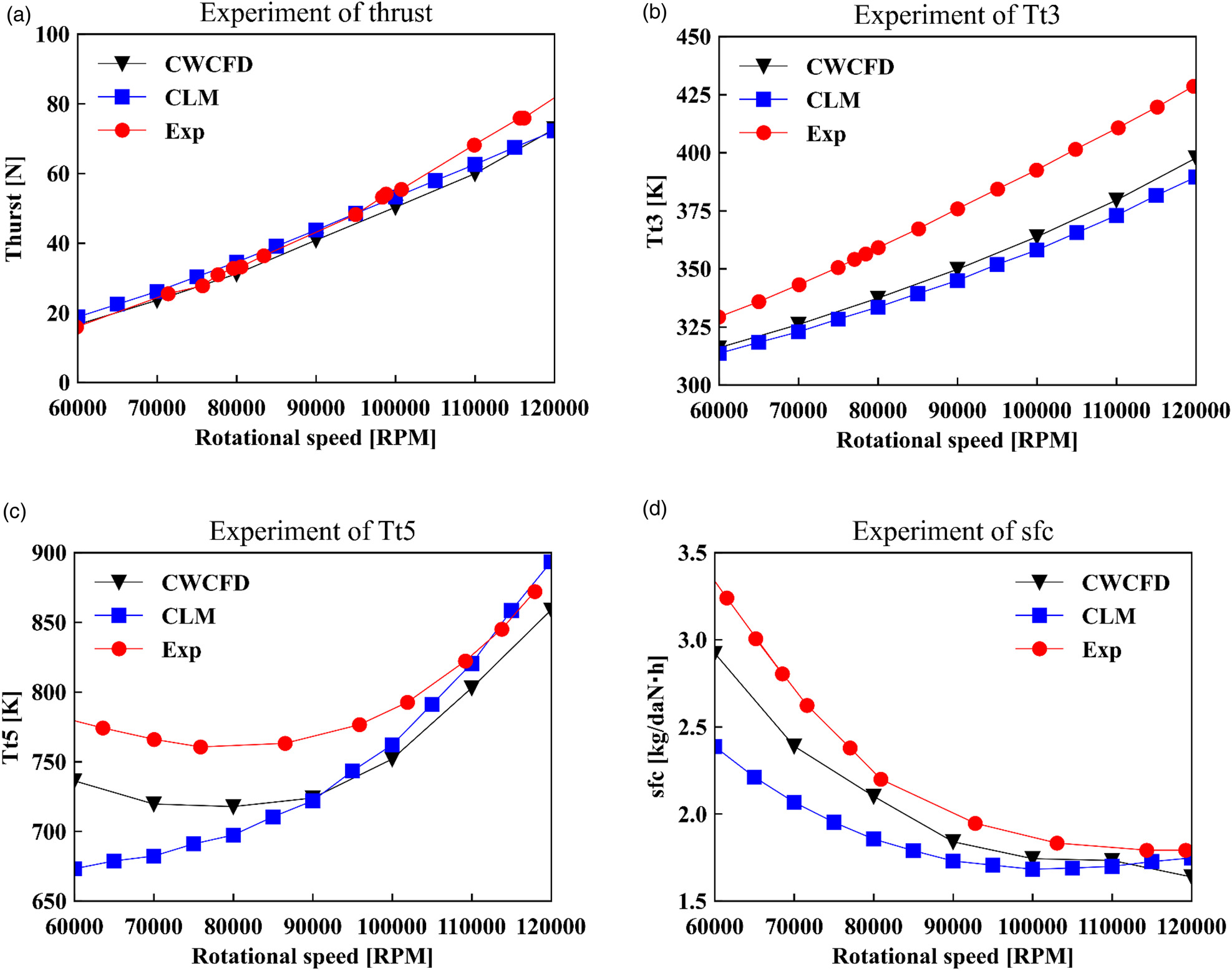
Table 3.
The global error of the throttle characteristic.
| Parameters | ||||
|---|---|---|---|---|
| CLM | 6.639% | 5.484% | 7.486% | 13.969% |
| CWCFD | 4.078% | 4.535% | 6.196% | 9.286% |
The accuracy of the component-level model is primarily dependent on the characteristic maps, which are generated under standard operating conditions corresponding to the design point. Due to their inability to capture detailed component information and real operating conditions, the characteristic maps can introduce some errors. Thus, extensive modification and correction are needed through experiments and expert knowledge, especially at the off-design point. In contrast, the CWCFD method operates without the need for characteristic maps. Moreover, each iterative solution of the equilibrium equations originates from CFD numerical simulations conducted under actual operating conditions. This intrinsic advantage results in high accuracy, even in off-design conditions such as the low-speed region. Consequently, the CWCFD method exhibits high accuracy, particularly in off-design conditions.
While the total number of iterations in the component-level model serves as an indicator of overall convergence behavior, it does not necessarily directly reflect the total simulation time. For instance, a single run of a component-level model achieves convergence within a relatively brief span of approximately 0.1 s. Therefore, the primary determinant of simulation duration is the creation of characteristic maps through CFD simulations. Consequently, the overall simulation time for a specific speed line within these maps is greatly influenced by the associated CFD simulations, each requiring 12 runs and contributing to an aggregate simulation time of 12 h. However, converging one operational point within the CWCFD model eventually took around 12 h, encompassing 12 iterations. Nonetheless, the improved accuracy of the CWCFD model at low-speed regions justifies the added computational cost.
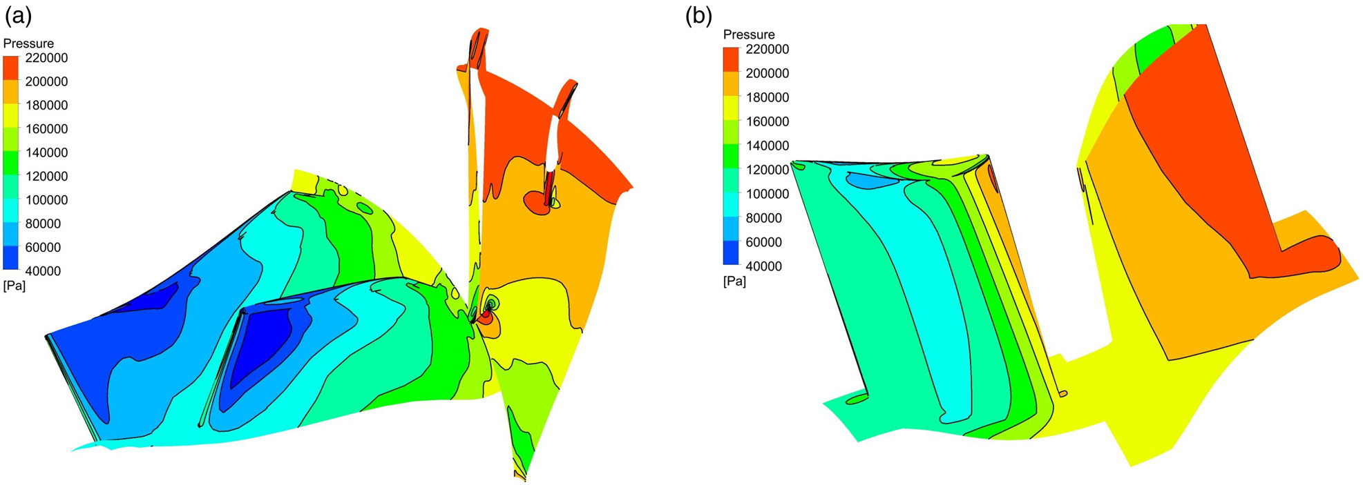
After analyzing the results, it was found that the CWCFD zooming method outperformed the CLM method in terms of accuracy. In addition, the CWCFD method also provided a more comprehensive understanding of the complex flow characteristics within the engine, as shown in Figure 5. This figure illustrates the detailed static pressure distribution of the compressor and turbine, which cannot be captured by the CLM method. Therefore, the CWCFD method is not only more accurate but also provides additional insights into the internal flow detail of the engine. This information is crucial for optimizing the engine's design and improving its performance. In summary, the CWCFD method offers a higher global accuracy of throttle characteristics and more detailed information than the CLM.
Conclusions
A CWCFD numerical zooming method was developed in this paper, which directly exchanges mass flow between CFD and CLM. The CWCFD zooming method is implemented by embedding multiple 3D CFD models of compressor and turbine (coaxial rotating) into a CLM instead of the corresponding characteristic maps, and it was applied to the simulation of the KJ66 MGT. The throttle characteristics, including a wide range of off-design points, are simulated. The CWCFD zooming method is compared with the traditional CLM method. Finally, the experimental data of the ground test are carried out to verify the effectiveness of the zooming methods. The results were analyzed in detail, and the performance of the CWCFD zooming method was found to be superior to the CLM method in terms of accuracy. However, the improved accuracy of the approach at low-speed regions justifies the added computational cost.
It is worth noting that the CWCFD zooming method eliminates the need for characteristic maps and correction between real conditions and ISA. Replacing the corrected mass flow and rotational speed with the actual mass flow and rotational speed avoids some computation errors from correction. Moreover, it allows the option of selecting independent variables of the cooperation equations as mass flow rather than the corrected mass flow, which simplifies the exchange of parameters between CLM and CFD models. The results suggest that the CWCFD zooming method is a promising alternative to future aeroengine design and optimization.