
Introduction
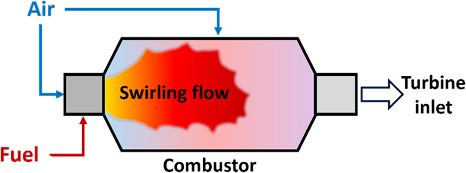
Swirling flow could always be found in the combustor of gas turbine or aircraft engine (Figure 1). Generated by the swirler, swirling flow is capable of improving the atomization condition, and stabilizing the combustion. Inevitably, the high thermal loads associated with the swirling jet often cause ablation of the combustor endwall, necessitating the design of effective thermal protection modules (Wurm et al., 2009, 2013). While the effective thermal protection modules are highly determined based on the swirling flow field. The accurate measurement of the swirling flow field is therefore crucial for the diagnosis of combustion stabilization and thermal protection. Furthermore, an accurate flow field is also important for optimizing combustion processes, improving efficiency, and reducing emissions.
Numerical investigations have been widely conducted from various perspectives (Xia et al., 1998; Spencer et al., 2008; Xiao and Zheng, 2014; Andrei et al., 2015). Although the numerical results revealed valuable three-dimensional mechanism of swirling flow to some degree, it was found that the numerical results weren’t always satisfactory. The recirculation zone, and swirling jet were always grossly predicted due to their inherent anisotropy (Jones et al., 2005) and the isotropic nature of the Boussinesq hypothesis used in numerical studies. In addition, another challenge for numerical simulation was that it was always difficult to obtain the expected results when the boundary conditions were unknown or deviated from the reality, which would always be applied when the boundary conditions were highly complex. Therefore, experimental investigations such as hot wire (Vu and Gouldin, 1982), laser Doppler velocimetry (Brum and Samuelsen, 1987), laser anemometry (Syred et al., 1994), and planar particle image velocimetry (PIV) (Andreini et al., 2014; Lenzi et al., 2022) could provide more accurate and reliable reference data, without knowing the boundary conditions. Besides for the flow field diagnosis, the cooling performance diagnosis of the common cooling design in the combustor, such as effusion cooling, slot cooling, was also widely conducted because of its most intuitive display of the cooling performance affected by the swirling flow (Andreini et al., 2014, 2015, 2017). In recent years, there have been researches investigating the effect of swirling flow on the cooling performance of cooling design based on the experimental observations, which have unveiled valuable flow and heat transfer characteristics (Jiang et al., 2022; Lenzi et al., 2023). However, the observations are always sparse or planar patterns due to the methodological limitations, resulting in the decreased three-dimensional analyticity. Therefore, leveraging experimental observations of swirling flow field would be beneficial for both scientific and industrial purposes. Inferring three-dimensional turbulent flow field through two-dimensional observations is a highly nonlinear mapping issue. Artificial neural networks, currently, are widely adopted fitting nonlinear functions for its outperformed capability to represent nonlinear mapping. To address this issue, Physics-informed neural networks (PINNs) have been proposed as a powerful approach to reconstruct three-dimensional flow fields from sparse or planar observations.
Designed by Raissi et al. (2018), PINNs have been widely developed in resolving inverse problem for various scenarios, such as material sciences (Lu et al., 2020; Shukla et al., 2020), chemistry (Pfau et al., 2020; Ji et al., 2021), geophysics (Li et al., 2020; Weiqiang et al., 2021), and topology optimization (Lu et al., 2021). PINNs also bring attentions to the field of flow and heat transfer for various scenarios. By inserting the prior knowledge of fluid mechanics such as continuity equation and Navier-Stokes (N-S) equations into the PINNs, the quantities in the domain field could be regressed. PINNs have shown the capabilities of leveraging the limited observations to reconstruct the laminar flow field. (Raissi et al., 2020; Cai et al., 2021a,c). For the turbulence problem, the Reynolds-averaged Navier–Stokes (RANS) method is adopted generally because of its higher efficiency and better convergence properties in numerical simulations. However, the derived term Reynolds stress, is unclosed yet, leading to the increased nonlinearity when resolving inverse problems for PINNs. Currently, the researches on RANS method are limited. Eivazi et al. (2022) evaluated the PINNs’ performance on the two-dimensional RANS equations without importing any turbulent viscous models. Cases of airfoil, periodic hill, etc. were applied, which validated that PINNs were capable of mining the latent mechanics of the turbulent model. Von Saldern et al. (2022) adopted the axis-symmetric swirling jet data and imported simplified Boussinesq hypothesis to evaluate PINNs’ regression on axis-symmetric RANS equations. They found that the velocity components were matched with the experimental results while the Reynolds stress components were poorly estimated. More complex cases of jet in crossflow were investigated by Huang et al. (2023), they designed the 2-rank tensor-basis eddy viscosity (t-EV) model to better fit PINNs’ structure and represent the anisotropy, effectively improving PINNs’ regression. It’s found from the above evidence that the investigated case is relatively simple and most of the training datasets are extracted from the clean numerical simulation. The performance of PINNs on predicting complex turbulent flow field haven’t been deeply evaluated, especially based on the experimental observations. Meanwhile, the observations from above researches only contain flow information. For the swirling flow in the combustor, scalar field is equally important as flow field. It’s believed that leveraging both scalar and flow field could further enhance the reconstruction performance, which also hasn’t been investigated yet.
The present work aims to reconstruct the complex swirling flow field based on limited experimental observations using PINNs. The effects of datasets on reconstruction are discussed preliminarily so that an effective sampling strategy is designed. Furthermore, the multi-source strategy would be adopted, where the scalar observation is introduced to improve PINNs’ prediction. Finally, the reconstructed vortex distributions would be shown to provide the evidences of the cooling performance destruction under swirling flow. The investigations in this study would provide the alternative to obtain the three-dimensional swirling flow field leveraging experimental observations with deep learning and deepen the understanding between the film cooling performance and swirling flow from a novel method, which is potentially beneficial for the cooling structure improvement in the future.
Methodology
Multilayer perception (MLP)
MLP is one of the essential parts of PINNs, which is a fully connected neural network. When MLP is being trained, the known input and output would be fed as the labels so that the parameters in neural network would be optimized to minimize the loss functions. Activation functions are added to increase the nonlinearity of the mapping. In this study, the mapping is expressed as:
where

Loss function
The loss functions of PINNs consist of two parts: loss functions of physics constraints and experimental observation. To obtained the mean flow field, the RANS equations are preparedly designed into the loss function of physics constraints:
The derived term
where Sij is the mean rate of strain tensor,
where
Thus, another six formulations would be designed into the loss function of physics constraints:
Note that the derivatives in these PDEs are obtained by automatic differentiation (AD) (Baydin et al., 2018). Therefore, the derivatives of these PDEs can be calculated by applying the chain rule under backpropagation. To satisfy these physical equations, the loss functions of physics constraints should approach zeros, which is formulated as
where Ne is the number of physical equations. Nd is the domain points in the selected regions.
For the observation loss functions, the two-dimensional and two-component (2D2C) results from PIV measurements are chosen as the labels, containing 2D2C mean velocities and their corresponding Reynolds stress. Furthermore, the non-slip boundary condition is added as known labels. Therefore, the loss function of the observations is reported as
The total loss then written by summing the weighted loss of above loss functions:
where

Multi-sources strategies
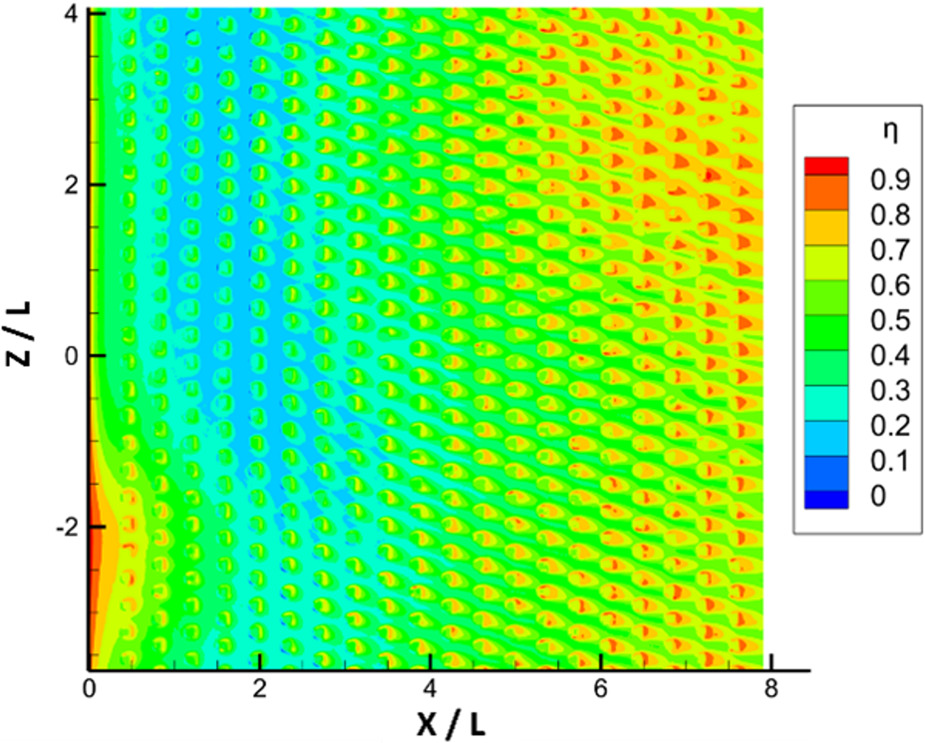
For the swirling flow in the combustor, scalar field is equally important as flow field. As the key variable to evaluate the film cooling performance, film cooling effectiveness was relatively measurable in the scalar field. Therefore, besides for the source from flow observation, the source from scalar field would also be imported to further improve PINNs’ regression. In this study, the scalar (i.e., film cooling effectiveness) observation of effusion plate is supplemented. The scalar distribution, as shown in Figure 4, is experimentally obtained by pressure-sensitive paint (PSP) measurement (Jiang et al., 2022). The PSP molecules could return to the ground state via the oxygen quenching process thus the cooling effectiveness could be acquired according to the calibrated luminosity-pressure correlation. The adopted 1,000 pairs of snapshots were captured for each case with a frequency of 1,800 Hz. The uncertainty of the PSP measurement was calculated to be around 2.7%.
The scalar equation is thus added into the loss function of physical equations:
where Pr is the Prandtl number, set as 0.71 in this study.
where
Dataset establishment
The dataset is established employing the PIV measurement (Jiang et al., 2022), where 1,000 pairs of snapshots were captured for each case. The spatial resolution of each snapshot was 0.023 mm/pixel with a frequency of 1 Hz. The uncertainty of the PIV measurement was calculated to be around 3%. As shown in Figure 5, seven observations were accessed during the measurement, containing two planes at XoZ direction (Y = 5 and 70 mm) and 5 planes (Z = 0, ±25.25, and ±50.5 mm) at XoY direction. In subsequent study, the coordinate is normalized, with a measured length L = 25.25 mm. To find out PINNs’ performance based on various number of observations, several training datasets are designed, as listed in Table 1. The two planes at XoZ direction are adopted throughout all datasets while the planes at XoY direction are increasingly sampled.

Results and discussion
Effect of sampling strategy on field reconstruction
Number of observations
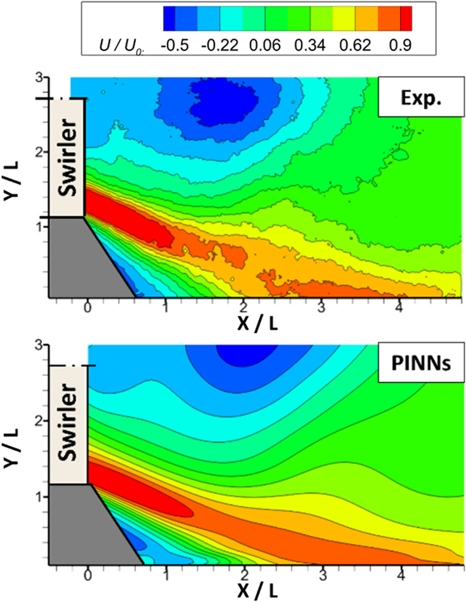
In this section, we focus on investigating the effect of the number of observations on reconstructing swirling flow, with the streamwise velocity as the main variable of interest. Following the sampling strategy employed in previous work (Cai et al., 2021b), sample 1 consists of four planes surrounding the regions of interest. However, unlike the well-reconstructed fields obtained in previous work, the performance of PINNs in predicting swirling flow fields is poor. As shown in Figure 6, (a) depicts experimental observations from PIV measurement, while (b) represents predictions made by PINNs using sample 1. It’s observed that the test dataset fails to capture the characteristics of the swirling flow, especially at the exit of the swirler, where the swirling jet should have emerged. Owing to the supplement of plane 1, the region where jet hit on the effusion plate could be predicted, but presented with shrunk area. This suggests that the vanilla sampling strategy is insufficient in leveraging the limited information provided by sample 1 to reconstruct complex swirling flow fields. It is therefore suggested that increasing the number of observations in the training dataset could improve the performance of PINNs. Subsequently, sample 2 and 3, which include additional information on the swirling flow field, will be adopted in the subsequent study.
Figure 6.
Comparison of streamwise velocity between (a) experimental observation and (b) prediction conducted by PINNs with sample 1.
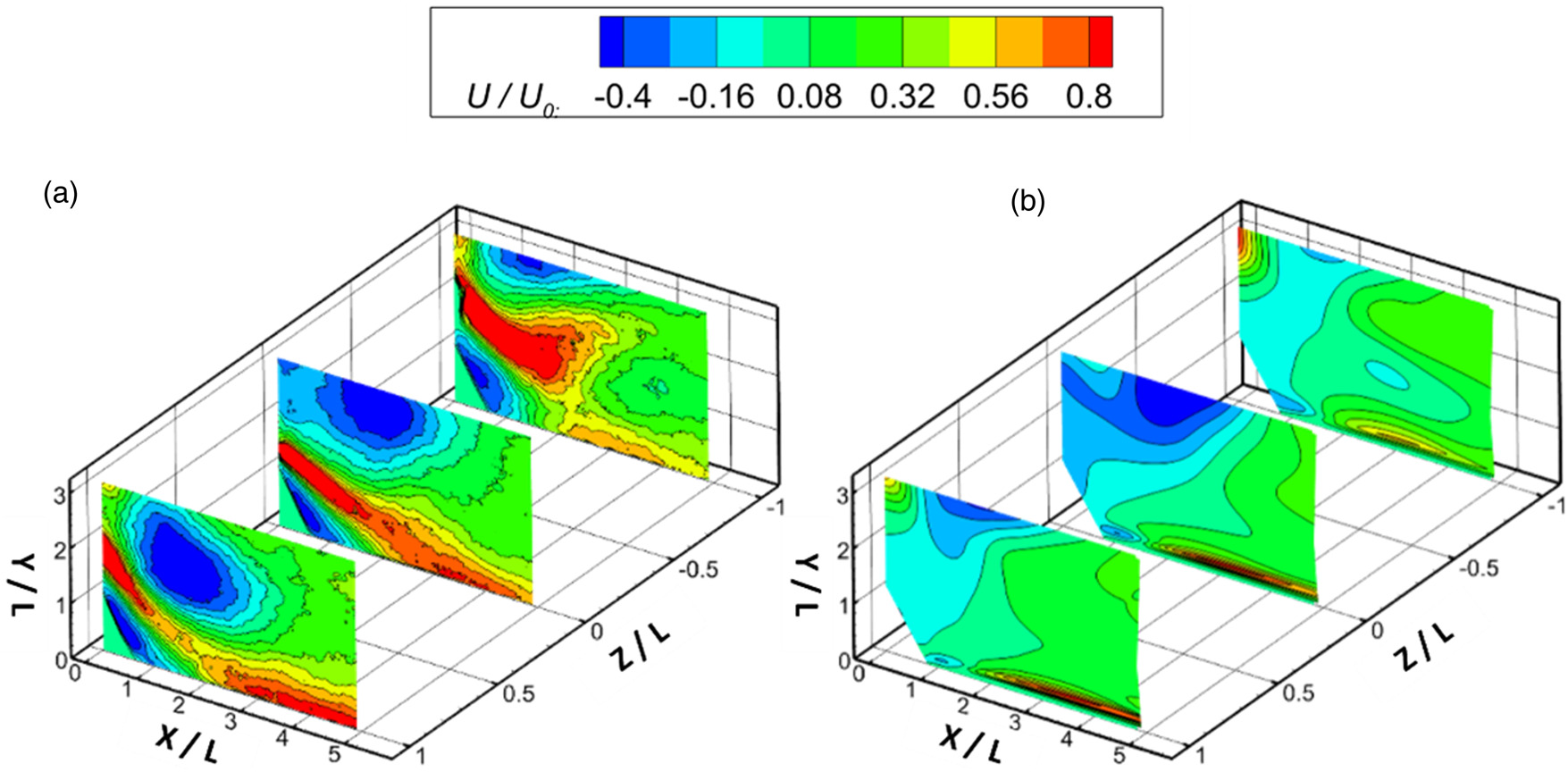
Figure 7 presents the predictions of PINNs using sample 2, where planes 4 and 5 serve as the test dataset. Compared to the predictions from sample 1, the overall performance shows improvement. Figure 6(a) shows that the jet at the exit of the swirler is captured for plane 4, although the velocity magnitude is weakened. However, a failed prediction is obtained for plane 5 in Figure 7b. The magnitudes of the recirculation zone and swirling jet at the swirler’s exit are much weaker than those of the experiments, as marked with red lines. In contrast, a better prediction is achieved when PINNs are trained with sample 3, as shown in Figure 8. The predicted streamwise velocity distribution of plane 3 shows satisfactory agreement with that of the experiment, including the recirculation zone, the jet at the swirler’s exit, and near the effusion plate. Furthermore, an improved denoise on the distribution could also be observed. Thus, the increasingly improved predictions suggest that compared to simple turbulent flow, swirling flow requires a higher number of fed observations to better capture the three-dimensional and complex swirling flow characteristics using PINNs.
Effective sampling strategy
From the results above, it can be concluded that the jet at the swirler’s exit is the most sensitive region to sampling strategies. In addition, Karniadakis et al. (2021) revealed that PINNs models often struggled on penalizing the PDEs residuals when tackling the solution with steep target gradients. Therefore, the regions with steep velocity gradients, such as the swirling jets, brought by the complex vortex structures and intense shearing would similarly increase the difficulty in PINNs’ accurate regression. Therefore, supplementing partial information at these sensitive regions can improve the prediction of PINNs. To improve the performance of PINNs, sample 1, which performed the poorest, was selected for investigation. In the updated sampling strategy, partial information containing the jet at the exit of the swirler was imported for planes 6 and 7 in the XoY direction, as shown in Figure 9a. The updated sample was named as sample 4. The predictions of PINNs with sample 4, shown in Figure 9b, indicate a significant improvement in the prediction of the unknown zones, such as the jet near the effusion plate and recirculation zones, compared with the poorly performing sample 1. However, it is also observed that the prediction of the jet highly close to the effusion plate is still unsatisfactory, where the streamwise velocity impinging onto the effusion plate is weakened. Statistically listed in the Table 1, compared with the poorly performed sample 1, sample 4 had the training volume of 106,308, where the additional observation of sample 4 reduced the numbers by 50% and 75%, respectively, compared with sample 2 and sample 3. To quantitatively analyse the PINNs’ performances in the test dataset of, relative L2 error is imported as the metrics, reported as:
Figure 9.
Scheme of sample 4, (a) is the sampling strategy, and (b) is the prediction conducted by PINNs with sample 4.

Sample 1 and 4 were chosen as the comparison due to the same test dataset. It was found that the relative L2 error of the test dataset has been effectively dropped from 0.84 to 0.24, with an reduction of 71.4%. Therefore, it can be concluded that the performance of PINNs for the prediction of complex swirling flow can be improved by increasing the number of observations, particularly in sensitive regions, to better capture the three-dimensional and complex characteristics of swirling flows.
Multi-source strategy
The scalar distribution of the effusion plate (shown in Figure 4) highlights the complex interaction between the effusion film and swirling flow. The low FCE zone is attributed to the mixing of swirling jets with the film, resulting in film coverage destruction. Supplementing observations of scalar sources prompts the PINNs to extract latent flow information and improve their performance.
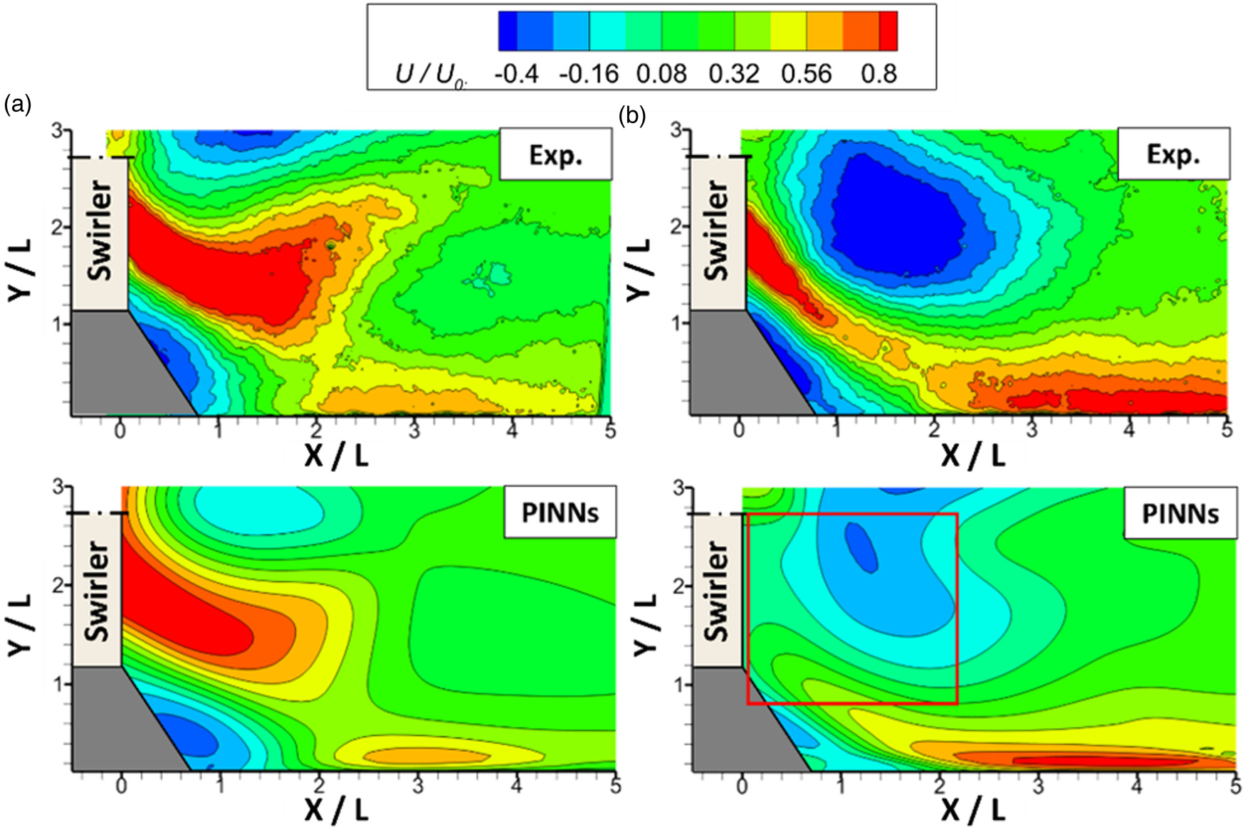
The investigation focuses on samples 2 and 4. In sample 2, the results in Figure 10 reveal improvements in the predicted flow below Y/L = 1. The regions marked by the red lines show more agreement with experimental observations, indicating a better distribution compared to the single-source strategy. For Plane 4 (Figure 10a), the marked zone is corrected as a higher velocity zone. While for plane 5 (Figure 10b), although the high streamwise velocity at the swirler outlet is not predicted accurately, the jet’s majority at the exit of the swirler agrees well with the experiments, indicating a better distribution than the single-source strategy. Note that the improvements propagating vertically are clearly reduced after Y/L > 1, where only limited correction could be observed, and the streamwise velocities of recirculation zone are still ill-matched with that of experimental observations. For sample 4, as shown in Figures 11a and 11b, the improvement is also observed, mainly for the marked regions near the effusion plate. To quantitatively analyse the amelioration provided by the multi-source strategy, the streamwise velocity profiles at the ill-performed marked region are shown in Figure 11c. It’s found that the more upstream zone shows the more noticeable improvement. For plane 5 (Z/L = 1), whose ill-prediction is concentrated in the downstream zone (Figure 9), the mean error of streamwise velocity weakly reduces from 18.7% to 13.5% after adopting multi-source strategy. While for planes 3 (Z/L = 0) and 4 (Z/L = −1), the improvements are obvious, where the mean errors are reduced from 18.1% to 6.9% and 6.8% to 1.6%, respectively. Note that the improvements for planes 5 and 3 near the jet impingement zone (Y/L < 0.5) are limited to some extents due to the insufficient downstream observations, suggesting that a satisfactory reconstruction of swirling flow field requires both designed multi-source and sampling strategies.
Figure 10.
PINNs’ prediction based on sample 2 with single source (top) and multi-source (bottom), validated by (a) plane 4 and (b) plane 5.
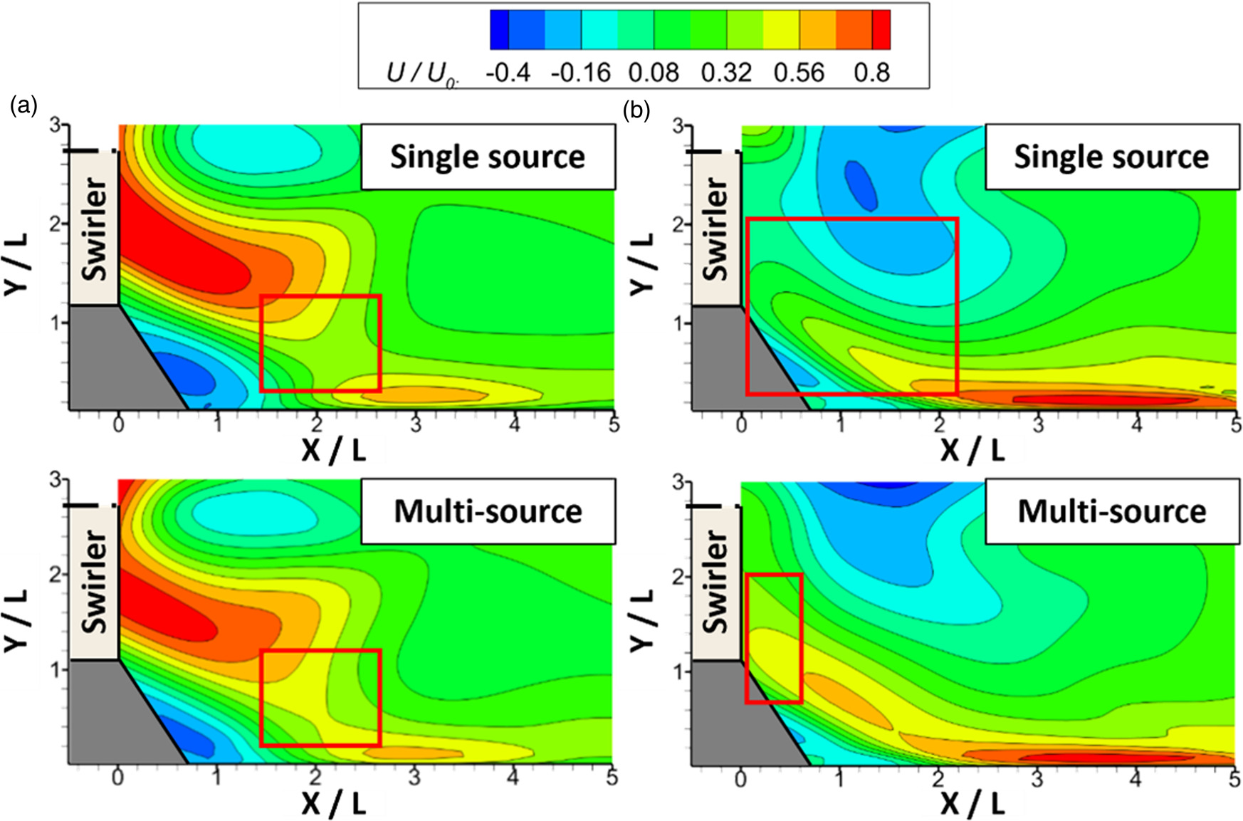
Figure 11.
PINNs’ prediction based on sample 2 with single source (a) and multi-source (b). (c) Are the quantitative comparisons of marked region for validation set.

To show the three-dimensional analysability of the reconstructed flow field, PINNs regression based on sample 4 and the multi-source strategy is selected as the investigation. As shown in Figure 12, the vortex structures are extracted from the predicted velocity field based on the Q criterion with a normalized value of 0.113. Note that only half of the vortex can be predicted because the PIV experiments only captured the half of the swirling flow field. The shown vortexes are found as a ring-like pattern similar with the previous literature (Chen and Driscoll, 1989; Oberleithner et al., 2011), named as recirculation vortex or recirculation bubble. The contours of vortexes in Figures 12a and 12b are marked by vertical velocity of Y direction and lateral velocity of Z direction, respectively. The black streamlines indicate the general swirling direction of swirling flow. The adiabatic cooling effectiveness is also shown. It’s found from the vortex structure distributions that the vortexes are mainly captured near the exit of the swirler (around 0 < X/L < 2.5), corresponding to the direct impingement region of the swirling jet in Figure 11b. From the contour in Figure 12a, it’s observed that the lateral velocity near the effusion plate is shown as negative value, indicating that the swirling flow would induce the effusion film deviating towards the opposite direction of the Z-axis. Therefore, the cooling effectiveness distribution presents the swept pattern. The region marked with the dashed red rectangle shows the obvious deviation of the cooling effectiveness distribution because of the strongest sweeping effect brought by the closest interaction of swirling flow. As the swirling flow develops downstream (2.5 < X/L < 4.5), there are still vortexes be recognized and marked as the negative lateral velocity, meaning that the swirling flow could continuously affect the effusion cooling and deviate the cooling effectiveness distribution. It’s then found from Figure 12b that both positive and negative values of vertical velocity are found as balanced distributions. The region with positive and negative value indicates that the swirling flow go through the upwash and downwash motions, respectively. It’s found near the exit of the swirler that the vertical velocity distributed as the negative value, revealing that the swirling flow downwards impacts and damages the surface of the effusion film, reducing the cooling effectiveness. Similarly, the region marked with the dashed red rectangle still shows the most severe deterioration of cooling performance than the surroundings due to the most direct impingement of swirling flow. Due to the occlusion of the vortex structures, it could be observed combining with Figure 4 that the effusion films at Z/L < −1 are less destructed due to the upwash motion of swirling flow. As the swirling flow develops downstream, the recognized vortexes are marked as weakly positive values. It is revealed that the swirling flow is slightly lifted off, meaning that the destructions on the cooling performance are gradually attenuated, thus leading to the recovery in cooling effectiveness.

Conclusions
In this study, the reconstructions of swirling flow field were conducted using PINNs fed by limited observations, where the observations of velocity and scalar were experimentally obtained. The sampling and ameliorated strategies were mainly investigated. Effects of the number of observations was firstly evaluated, it was found that the reconstruction improved as the number of observations increased. Based above, zones of swirling jet show the high sensitivities towards number of observations. To optimize the dataset, the effective sample 4, containing the partial swirling jets with complex vortex structures and intense shearing (i.e., steep velocity gradients region) was designed by reducing the additional observation by 50% and 75% compared to sample 2 and 3, respectively, still resulting in a well-reconstructed flow field. Compared with sample 1, the relative L2 error of sample 4 showed an effective reduction of 71.4%.
To further improve the PINNs’ prediction, the multi-source strategy was employed by supplementing the observations from the scalar field into PINNs. Additional prior knowledge of scalar transportation was also supplemented into the loss functions. The sample 2 and 4 were selected as the investigations. It was found that the prediction of swirling jet for sample 2 was obviously improved. For sample 4, statistically compared with the previous, the mean errors of streamwise velocity at the marked region were reduced by 61.9%, 76.5%, and 27.8% for plane 3, 4, and 5, respectively. The supplementary scalar distribution was assumed to strengthen the latent information of the complex interactions between swirling flow and the effusion film.
Finally, the three-dimensional analysis of the reconstructed flow field unveiled that swirling flow vortex structures presented a crucial role in cooling effectiveness. It was found that these vortexes, especially near the swirler exit, significantly impacted the cooling performance, inducing a swept and deteriorated pattern in the cooling effectiveness distribution. As the swirling flow developed downstream, the vortexes’ influence on cooling effectiveness gradually attenuated, leading to a recovery in cooling performance. From the engineering perspective, it is advisable to allocate a greater proportion of coolants or design a more effective cooling structure to the region near the swirler exit, especially near the central side following the swirling flow direction.
The investigation in this study explored the method on reconstructing complex turbulent flow field using deep learning based on the experimental results, which provided the alternative for diagnosing the complex flow and ameliorating flow field. This reconstructed turbulent flow and vortex field highlighted the intricate relationship between vortex structures and cooling effectiveness, which intended to deepen the understanding of effusion cooling under swirling flow condition from a novel method. Considering that the investigated region was the swirling flow field, the more complex phenomena haven’t been captured accurately, such as the chemical reactions and the interactions near the wall between swirling flow and effusion film. In addition, the current study still required a large volume of data for a satisfactory flow field reconstruction. Therefore, the methodology proposed in this study was not intended to substitute the numerical simulation or other three-dimensional experimental diagnosis. It was aimed to propose one solution to leverage the existing but limited observations to potentially improve the flow field analysability for both scientific and engineering purposes. Future studies would focus on finer reconstruction of the complex turbulent wall-bounded flow. Furthermore, due to the PINNs regression is a case-by-case process. Future studies would also focus on the acceleration for PINNs with more efficient designed deep learning structure.