0D ACE performance simulation

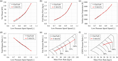
The 0-D ACE performance model is developed in Matlab and Simulink platform based on object-oriented programming technology, using the open-source package T-MATS (Toolbox for the Modeling and Analysis of Thermodynamic Systems) released by NASA Glenn Research Center (Chapman et al., 2014). Because no engine test data is available to validate the established model in this paper, the trust in the model accuracy is placed on the soundness of the developed modeling methodologies and the results, which showed expected trends for the most part (Kopasakis et al., 2015). For the above purposes, two validation cases are presented to demonstrate the accuracy of the 0D performance modeling methodologies. The first case is the performance comparison between the test and T-MATS data for a mixed-flow turbofan engine, as shown in Figure 1. All the parameters are normalized by the corresponding test value at 100% design speed. In the modeling, the performance maps of the fan, HPC, HPT, and LPT were obtained from the component tests. It is found that the performance deviations between the test data and T-MATS data are less than 2%, and the trends of all the performance changes with the low-pressure spool speed predicted by T-MATS agree well with those of the test. Although the ACE and the mixed-flow turbofan engine are different in configuration, the results indicate the reliability of the modeling methodologies on the multi-stream engine to some extent. The second case is the performance comparison between the commercial software GasTurb (Kurzke and Halliwell, 2018) and T-MATS for the double-bypass variable cycle engine with the F120 engine configuration. As shown in Figure 2, the key performance parameters, including thrust, fuel mass flow, turbine inlet temperature (T4), and bypass ratio, as well as the operating lines predicted by T-MATS, agree well with those of GasTurb, except for the large thrust deviation at the low rotational speed caused by the different mixer modeling method, which proves the validity of the modeling methodologies.

Figure 1.

Mixed-Flow Turbofan Engine Performance Comparison between Test and T-MATS. (a) Net Thrust, (b) Fuel Mass Flow, (c) LPT Outlet Temperature T5, (d) Bypass Ratio, (e) Total Pressure Ratio, and (f) Operating Line on Fan Map.

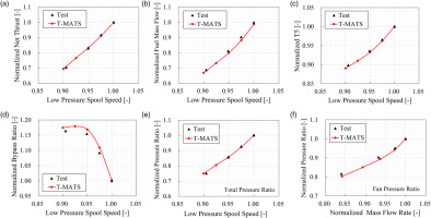
Figure 2.

Double-bypass variable cycle engine Performance Comparison between GasTurb and T-MATS. (a) Net Thrust, (b) Fuel Mass Flow, (c) Turbine Inlet Temperature, (d) Total Bypass Ratio, (e) Operating Line on Fan Map, and (f) Operating Line on CDFS Map.

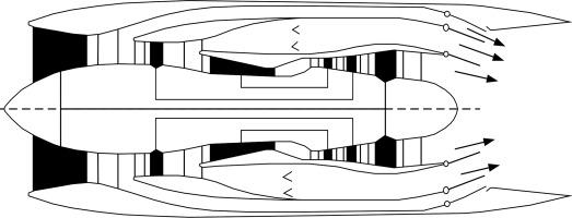
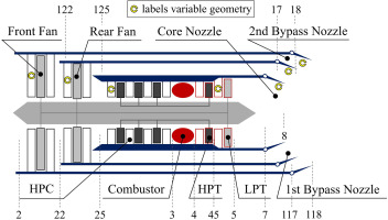
The modulating bypass (MOBY) variable cycle engine configuration was proposed by General Electric in the 1970s (Johnson, 1995), as shown in Figure 3, which laid an important foundation for the development of variable cycle engines and ACEs. The MOBY consists of three spools, two-section split fans, the duct burner, and three variable separated flow nozzles, which are highly complex in structure. In this paper, an ACE with a three-stream configuration is selected for study, and the schematic diagram is shown in Figure 4. Compared with MOBY, the three-spool configuration is replaced by the two-spool configuration, the two-section split fans are on one spool, and the duct burner is removed in this ACE. The ACE consists of the adaptive fan which includes the front fan and the rear fan, the HPC, the combustor, the HPT, the LPT, the core nozzle, the first bypass nozzle, and the second bypass nozzle. The guide vane or stator vane angle of the front fan, rear fan, HPC, HPT, LPT, and the throat areas of three nozzles are adjustable, as shown in Figure 4. To represent the effects of variable geometry on the component characteristics, multi-angle characteristic maps (Sullivan and Parker, 1979), which contain information on the mass flow rate, pressure ratio, and isentropic efficiency under different guide vane angles, are used for the front fan and rear fan, and the empirical relations (Edmunds, 1977; Grönstedt, 2000) to predict the maps with changed guide vane or stator vane angle are used for the HPC, HPT, and LPT.

Figure 3.

Three-Spool Double Bypass MOBY.

Figure 4.

Three-Stream ACE Configuration.

The design point of ACE is selected at sea level and static state, and the main parameters at the design point are shown in Table 1. The front fan split ratio is equal to the ratio of the mass flow rate in the second bypass duct to the mass flow rate in the rear fan. The rear fan split ratio is equal to the ratio of the mass flow rate in the first bypass duct to the mass flow rate in the HPC. The iteration and error variables of ACE to reach the convergence of equations based on the matching of each component at the off-design point are shown in Table 2. The low-pressure spool speed is set, and the Newton-Raphson iterative method is adopted to calculate the off-design point performance.

1D adaptive fan and 1D LPT mean-line analysis

The turbomachinery 1D mean-line analysis approach plays an essential role in the engine conceptual and preliminary design stage due to its simplicity and rapidity. Compared with the scaled generic characteristic maps in the 0D ACE model, the characteristics from the 1D mean-line analysis are usually with higher accuracy and fidelity, because it is a physics-based approach. The effects of the variable guide vane/stator vane, tip clearance, and other second-order effects on the engine performance can be taken into account in detail.

The accuracy of the 1D mean-line analysis mainly depends on the loss and deviation models. Many empirical correlations for the loss and deviation models have been proposed by researchers in turbomachinery, based on a great amount of cascade test data. However, these models are commonly suitable for the early standard blade profiles and can obtain good performance prediction accuracy in the low-speed turbomachinery. On the other hand, with the development of turbomachinery design technology, advanced three-dimensional blade profiles have been widely used in high-performance turbomachinery. Therefore, the early proposed model coefficients need to be updated to meet the performance prediction requirements with the changed turbomachinery design strategy.

The 1D adaptive fan and 1D LPT mean-line analysis approach adopted in this paper are developed in the literature (Song et al., 2022) and (Wang et al., 2022), respectively. In both literatures, the empirical coefficients of the loss and deviation models are optimized based on the performance test results of multiple cases. The genetic algorithm is adopted for optimizing the empirical coefficients in the loss and deviation models. Hausdorff distance is employed for quantifying the discrepancy between the test and 1D prediction performance, which is taken as the optimization objective function. The optimized profile loss model and deviation model are briefly described below.

In the 1D adaptive fan mean-line analysis approach, the off-design profile loss model is shown in Equation (1), and the deviation model is shown in Equation (2). The empirical coefficients of both models are optimized from the Creveling model (Creveling and Carmody, 1967). In Equation (1), ω, i, and M_in denote the profile loss coefficient, incidence angle, and inlet Mach number, respectively. The subscript ref denotes the parameters in the reference state. In Equation (2), δ denotes the deviation angle, ε denotes the flow turning angle, and x is a function of i, i_ref, and ε.

In the 1D LPT mean-line analysis approach, the off-design profile loss model is shown in Equation (3), the empirical coefficients of which are optimized based on the Kacker and Okapuu model (Kacker and Okapuu, 1982), and the deviation model is shown in Equation (4), the empirical coefficients of which is optimized from the Zhu and Sjolander model (Zhu and Sjolander, 2005). In Equation (3), i_stall means the stalling incidence angle. In Equation (4), γ, c, β₁, β_1m, β_2m, t_max, Re denote the stagger angle, chord length, inlet flow angle, inlet metal angle, outlet metal angle, maximum blade thickness, and Reynolds number, respectively.

Multi-fidelity ACE performance simulation

A multi-fidelity ACE performance simulation model is established in this section by integrating the 1D front fan mean-line analysis model, 1D rear fan mean-line analysis model, and 1D LPT mean-line analysis model into the 0D ACE model with the iteratively-coupled method. The advantage of the iteratively-coupled method is that the data from the 0D ACE model to the 1D adaptive fan and the LPT model can be transferred in both directions, respectively, without changing the mathematical model and architecture of the 0D ACE model, compared with the fully-coupled method.

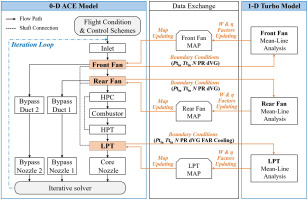
The 0D/1D iteratively-coupled simulation process is shown in Figure 5. First, the flight conditions and engine control schemes are set, and 0D ACE simulation is carried out with the Newton-Raphson iterative solver to obtain the components’ boundary conditions. The boundary conditions of the front fan and rear fan include the inlet total pressure Ptin, inlet total temperature Ttin, low-pressure spool speed N, total pressure ratio PR, and guide vane angle variation dVG, and the boundary conditions of the LPT include fuel air ratio FAR, cooling parameters in addition to those of the adaptive fan. Then the 1D front fan, 1D rear fan, and 1D LPT mean-line analysis are conducted to obtain the 1D performance of each component. Based on the results of the 0D ACE model and 1D turbomachinery models, the residuals of each component’s mass flow rate W and the isentropic efficiency η are generated. When the residuals do not satisfy the convergence criterion, a set of correction factors of W and η are calculated, which are used to update the scaling factors of the front fan, rear fan, and LPT generic characteristic maps in the 0D ACE model. The above process is repeated until all the W and η residuals satisfy the convergence criterion. To realize the automatic data transfer in the iteratively-coupled simulation, the 0D ACE model constantly calls the executable files of the 1D adaptive fan models and the m-file of the 1D LPT model.

Figure 5.

0D/1D Iteratively-Coupled Simulation Flow Chart.

The residual Res can be calculated from Equation (5), where the subscript 1D denotes the parameters calculated by the 1D turbomachinery models and 0D denotes the parameters calculated by the 0D ACE model. The convergence criterion is that the residuals of each parameter do not exceed 1 × 10⁻⁴.

The scaling factors of the mass flow rate f_W and efficiency f_η are calculated by Equation (6), referring to the literature (Klein et al., 2017), where i and i−1 denote the parameters of the current iteration step and the previous iteration step, respectively, and δ denotes the relaxing factor, used to suppress the residuals oscillation. In this paper, δ is set to 0.5.

Effect of component zooming on engine performance and computing time

The developed multi-fidelity ACE simulation approach enables free switching of the component dimension between 0D and 1D, realizing the component zooming function.

The performance comparisons of the multi-fidelity ACE models with different component zooming strategies are shown in Figure 6.

Figure 6.

Performance Comparisons of Multi-Fidelity ACE Models. (a) Net Thrust, (b) Specific Fuel Consumption, (c) Turbine Inlet Temperature, (d) Total Bypass Ratio, (e) Operating Line on RFAN Map, and (f) Operating Line on LPT Map.

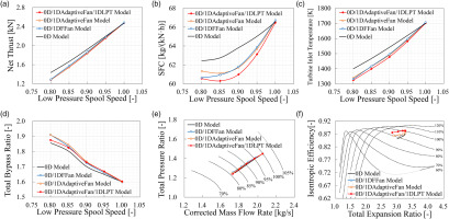
The legend 0D/1DFFan Model denotes the results of coupling the 1D front fan model with the 0D ACE model, the legend 0D/1DAdaptiveFan Model denotes the results of coupling the 1D front fan and 1D rear fan model with the 0D ACE model, and the legend 0D/1DAdaptiveFan/1DLPT Model denotes the results of coupling the 1D adaptive fan and 1D LPT model with the 0D ACE model. RFAN denotes the rear fan. When the low-pressure spool speed is lower than 90% speed, the throat area of the second bypass nozzle increases by 8% to increase the front fan surge margin. As shown in Figure 6, the performance of the multi-fidelity models and 0D model at 100% low-pressure spool speed is basically the same, but the performance deviations increase as the speed decreases. Among all the multi-fidelity models, the 0D/1DAdaptiveFan/1DLPT model deviates the most from the 0D model regarding thrust, SFC, and T4. Compared with the multi-fidelity models, the 0D model overestimates the thrust, SFC, and T4, but underestimates the bypass ratio. The maximum deviations of thrust, SFC, T4, and bypass ratio between the 0D/1DAdaptiveFan/1DLPT model and 0D model are −10.8%, −4.4%, −5.4% (−75 K), and 1.6%, respectively, which are considerable and non-negligible for the application in the design stage of ACE.

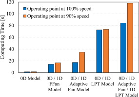
The computing time comparisons of different multi-fidelity ACE models at 100% and 90% low-pressure spool speeds are shown in Figure 7. FFAN denotes the front fan. The computing time of the 0D model is about 1.5 s. Due to the adoption of the 1D turbomachinery models and iteratively-coupled simulation, the computing time of the multi-fidelity models increases obviously. As the speed decreases, the component characteristic differences between the multi-fidelity models and the 0D model increase. Therefore more iterations are required, resulting in more computing time for off-design speed than for design speed. However, the computing time of this magnitude is short enough and quite acceptable to be applied in the preliminary design stage, compared to that of the massively parallel computation of the three-dimensional computational fluid dynamics (CFD) simulation. The computing time of all the multi-fidelity models is less than 2 min, and the main time spent comes from calling and running the 1D LPT model, which will be optimized to further reduce the computing time.

Figure 7.

Computing Time Comparisons of Multi-Fidelity ACE Models.

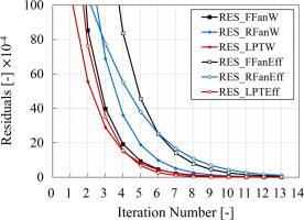
The variations of the residuals with the number of iterations at 90% low-pressure spool speed are shown in Figure 8. After 13 iterations, all the residuals meet the convergence criterion.

Figure 8.

Variations of Residuals with Iterations.

Effect of variable guide vane angle on engine performance

With the multi-fidelity models, the effect of variable guide vane angle on the engine performance can be evaluated. The 0D/1DAdaptiveFan/1DLPT model, abbreviated as the MD model, will be used for performance analysis in this and subsequent sections.

The effect of the rear fan inlet guide vane (IGV) angle on the engine performance at 100% low-pressure spool speed is shown in Figure 9, and the deviations between the MD model and 0D model are also presented. The negative angle indicates that the IGV is opened. As the rear fan IGV angle decreases from 0°, the rear fan mass flow rate and pressure ratio increase, leading to the increment of the rear fan power. The fuel consumption needs to be increased to keep the low-pressure spool operating at 100% speed, resulting in the increased T4 and thrust. As shown in Figure 9, the thrust, SFC, and T4 predicted by the 0D model are lower than those of the MD model, and when the rear fan IGV angle is set to −12°, the deviations are 4.5, 4.7, and 4.9% (85 K), respectively. The multi-fidelity simulation approach proposed in this paper can also evaluate the effect of the variable geometries of multiple IGVs and stators on engine performance.

Figure 9.

Effect of Rear Fan IGV Angle on Engine Performance at 100% Low-pressure Spool Speed. (a) Net Thrust, (b) Specific Fuel Consumption, (c) Turbine Inlet Temperature.

The effect of the LPT IGV angle on the component and engine performance at 90% low-pressure spool speed is shown in Figure 10 and Table 3, respectively. The two-stage LPT is utilized to fulfill the design value of the LPT expansion ratio equal to 3.2. IGV1 means the first stage IGV, while IGV2 means the second stage IGV. Similar to the adaptive fan, the negative angle indicates that the IGV is opened. In Figure 10, the operating points when IGV1 = −4°, 0°, 4° are shown on the component maps. As the LPT IGV1 angle decreases, the LPT flow capacity increases, resulting in a decrement in the LPT expansion ratio and an increment of the HPT expansion ratio. As a result, the high-pressure spool speed increases, the bypass ratio decreases, and the back pressure of the front fan and rear fan decrease, leading to the operating points moving away from the surge boundary. In Table 3, the decrement of the LPT IGV1 results in the increment of the thrust and SFC, while the LPT IGV2 shows little effect on the performance, indicating that the aerodynamic throat of the present LPT design locates at the first stage.

Figure 10.

Effect of LPT IGV1 Angle on Component Performance at 90% Low-pressure Spool Speed. (a) Operating Point on FFAN Map, (b) Operating Point on RFAN Map, and (c) Operating Point on LPT Map.

To realize the switching of operating modes and the optimal performance in different modes, the ACEs require its components to have the capability of wide-range variable geometry, which brings a significant challenge for the ACE performance prediction with high accuracy. The multi-fidelity simulation approach proposed in this paper is a good tool to cope with the challenge above under the acceptable computing resources and time cost.

Effect of tip clearance on engine performance

Tip clearance is an intriguing and challenging topic in the development of aero-engines. Too large or small tip clearance will significantly affect the engine performance and operation safety. With the MD model, the effect of tip clearance on the engine performance can be evaluated, which usually cannot be appropriately considered in the 0D model.

The effect of the LPT tip clearance on the engine performance at 100% low-pressure spool speed is shown in Table 4. The performance prediction model with changed tip clearance adopted here is from the literature (Agromayor and Nord, 2019). Because the engine mass flow rate is quite low, the ratio of tip clearance to blade height is large, resulting in a significant effect of the tip clearance on the LPT efficiency. The increase in the tip clearance leads to a decrease in the LPT efficiency and an increase in the SFC and T4. As the tip clearance increases, the performance deteriorations tend to slow down.

Subscript