
Introduction
Stall flutter occurs at part-speed regime, when airfoils operate at an incidence higher than nominal (Dowell, 2015); it is normally associated with high steady loading and low reduced frequency, for blades vibration in the first flap (1F), sometimes referred to as flapwise bending (also simply bending), or torsion (1T) mode (Srinivasan, 1997), in forward travelling assembly modes, with positive low nodal diameters from
For the flow driven mechanism, the inception of stall itself is not a necessary condition, though the flow separation, and its interaction with the suction side shock wave, is a key component for this type of instability. On the other hand, the acoustic driven mechanism is driven by the interaction of blade vibration with an upstream running wave caused by the blade vibration itself and the reflected wave from the intake. These conclusions are confirmed by a number of previous and subsequent studies.
Isomura and Giles (1998) carried out a numerical study of a transonic fan and concluded that the source of the instability is the shock wave/boundary layer interaction (SBLI) which primes the shock to oscillate, destabilising the blade. Vahdati et al. (2001) also performed a numerical study on a different fan blade, finding that actually the shock wave has a stabilising effect, while the opposite is true of the flow separation. It is therefore clear that these flow features can both exacerbate and eradicate flutter, depending on geometry, flow field, modeshape and frequency. Vahdati et al. (2011) carried out a numerical campaign to investigate the mechanism of wide-chord fan flutter. They found that SBLI only is not sufficient to explain the loss of stability near stall, and that this event is driven by acoustic waves propagating upstream being reflected at the intake highlight. They name this loss of stability “flutter bite”. Vahdati and Cumpsty (2015) performed a numerical analysis of a state-of-the-art fan blade, and concluded that flow separation, followed by radial migration of flow along the span towards the casing, decreases aerodynamic damping. They found that aerodynamic damping reduces as the twist component in the first flap mode increases, similar to what Panovsky and Kielb (1999) concluded for turbines. Finally, they state that flutter occurs in the frequency and nodal diameter range where the generated acoustic waves are cut-on upstream and cut-off downstream.
Building on this knowledge, Stapelfeldt and Vahdati (2019) presented two strategies to improve the flutter margin of an unstable fan blade. The first addresses the flow driven mechanism by restaggering sections of the blade, so that the radial pressure distribution is altered and the flow separation, with consequent radial flow migration, is mitigated. The second strategy involves bleeding a small amount of fluid at different chord locations, in order to attenuate the upstream running pressure wave from trailing edge to leading edge, thus addressing the acoustic driven mechanism. Finally, Rendu et al. (2019) presented a radial decomposition method of the blade vibration to identify the flutter source of a fan blade. They show that the fan blade is rendered unstable due to the highly destabilising contribution of the tip section of the blade, where the separation is most severe. By dividing the blade into radial panels and vibrating them individually, they found that the instability though is not caused by the tip itself, but rather is the vibration of lower panels that induces a destabilising unsteady pressure on the tip.
The challenge of predicting compressor flutter lies in the complex interactions between aerodynamic flow, structural mechanics and aeroacoustics which involves a large number of parameters. Analytical and computational methods for the prediction of compressor stall flutter have reached maturity, and development of new efficient techniques seems to have come to a halt. Machine learning offers a large set of tools to explore and model complicated phenomena with many variables involved, and it has proved successful in turbulence modelling, bridging the gap between closure models and high fidelity methods in a number of applications.
Data-driven models for fluid mechanics applications, though, often share a fallacy: they are not reusable, as predictions for the quantities of interest are only possible on training geometry or flow condition. The difficulties with extrapolation from the training space are well known in machine learning and efforts have been made to address these limitations with varying degrees of success. All the paradigms are based on introducing physical or domain knowledge into the process, and a brief summary of such approaches is in order to justify the choices made in this work.
Raissi et al. (2019) introduced the physics informed neural network (PINN) concept and applied it to solve a number of problems, including two dimensional shedding around a cylinder. The PINN framework includes the differential form of the governing equations, and relative boundary conditions, as loss terms inside the cost function so that predictions are consistent with the underlying physical problem, allowing the model to extrapolate to unseen conditions. However, even in their state-of-the-art form, PINNs have only been applied to relatively simple fluid flow problems (Jin et al., 2021; Oldenburg et al., 2022) and, more importantly, are still geometry dependent, i.e. a model trained on one geometry cannot be used on another.
Physical understanding can be incorporated through domain knowledge as well. Manepalli et al. (2019) built a model to predict snow accumulation on mountains and have incorporated certain domain knowledge via additional penalty terms into the cost function, which penalise the model for predicting snow accumulation on water surfaces. Daw et al. (2020) used an LSTM to predict lake water density and, as density can only increase with depth, they constrained their model to only predict monotonic, increasing trends. Frey Marioni et al. (2021) seeked to improve the modelling of the eddy viscosity term in the Boussinesq assumption, using neural networks trained on DNS data, with the ultimate goal of improving flow field predictions in a turbomachinery cooling flow. Rather than directly training on the complicated flow, they approximated it with a serpentine passage and employed hierarchical agglomerative clustering to classify and divide flow regions. They showed improved results by training only on regions without flow separation. Frey Marioni et al. (2022) built on their work to model wakes in an LPT cascade. Once again they showed that dividing the domain into simpler subdomains and employing clustering improves the predictive capabilities of their ML models.
Particularly in turbulence modelling, physical knowledge is incorporated in the formulation of meaningful input features. Ling and Templeton (2015) developed a number of classifiers to identify regions of high uncertainty in RANS computations, and ensured that the models had good generalisation properties by providing several features that are rotationally invariant and based on physical intuition. Their set of features has since been adopted by other researchers (Wang et al., 2017; He et al., 2022).
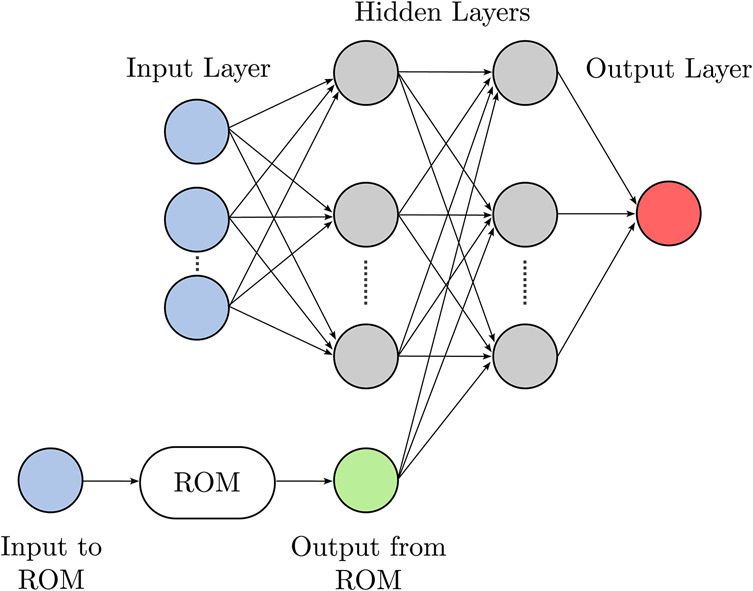
Finally, Pawar et al. (2021) introduced the concept of physics guided machine learning (PGML) and applied it to the prediction of lift coefficient on 4 and 5 digits NACA airfoils. The PGML framework in this case refers to a fully connected neural network (FCNN) where, at some hidden layer, results from a reduced order model (ROM) of the process are injected, thus augmenting the knowledge of the algorithm and “guiding” it to a physically consistent formulation. The same framework has been applied to modelling of dynamical systems with good degree of success Robinson et al. (2022), and both studies show good generalisation properties. This framework is appealing as it is computationally inexpensive, easily implemented, builds incrementally on previous, physically sound knowledge and acts as a regulariser, avoiding excessive overfitting even in a small-data regime.
Considering the discussion above, we seek to build a machine learnt model using the PGML framework with meaningful input and output features, based on physical understanding of stall flutter. Each component of the PGML model developed in this work will now be discussed.
Methodology
Flow solver
In this study, the data necessary to build our PGML model are obtained solely with computational methods. The CFD solver used in this work, LUFT, is developed by Dr. Paul Petrie-Repar from RPMTurbo. The steady-state solver employs a cell-centered finite volume scheme to solve the 3D RANS equations, on a computational grid composed exclusively of hexahedral elements. The fluxes are calculated by means of an upwind AUSM scheme and, at cell interfaces, the flow is reconstructed with a MUSCL interpolation coupled with the van Albada limiter. Finally, a pseudo-time stepping with residual smoothing is applied to march the solution to convergence.
The unsteady flow solver is linearised. The time dependent flow equations are cast in the frequency domain, so that the flow is assumed to be harmonically oscillating about its steady-state
Test case
The test case selected for this study is the Standard Configuration 10 (Frannson and Verdon, 1991), a 2D compressor cascade which consists of modified, cambered NACA
The grid used for both steady and unsteady computations is quasi-2D, i.e. one cell layer along the span, it has been obtained through a convergence study and it consists of
Machine learning algorithm
The backbone of the PGML model is a fully connected neural network. The choice of an FCNN is motivated by its layered structure, which allows full control over the location where the low-fidelity results are injected. A schematic representation of the FCNN is given in Figure 1.
Figure 1.
A schematic representation of a PGML network with two hidden layers and one-dimensional output.
A number of hyperparameters need to be specified now to build the model, such as number of hidden layers, number of neurons per hidden layer, regularisation coefficient, bias value, number of iterations, minibatch and step size, activation function and location of low-fidelity results injection. In this case, a full factorial exploration is unfeasible to say the least, therefore the standard practice of random search is employed. A set number of FCNNs will be trained with hyperparameters chosen randomly within pre-established ranges; the loss metrics are evaluated and the best models are then selected for a posteriori assessment.
In this work, we aim for small, simple FCNN architectures, therefore a large number of hyperparameters can be tested in parallel, even on conventional CPUs. The optimisation algorithm is Adam (Kingma and Ba, 2014), and the cost function is the standard mean squared error (MSE). The model is implemented in PYTHON with the TENSORFLOW (Abadi et al., 2015) library.
Reduced order model
The reduced order model we are seeking must:
- be efficient, thus adding minimum computational effort
- take into account some, if not all, geometrical features of the cascade
- model compressibility effects, due to the Mach number range of interest for stall flutter
- be validated
Output formulation
The same coefficients computed by LINSUB can be calculated using CFD. Two computations are necessary to calculate the unsteady pressures induced by each mode, which are consequently integrated along the blade to find forces and moments. Equation (2) shows the definition of two of the coefficients, for sake of brevity. The superscript refers to the mode causing the unsteady loads, while the subscript refers to the modal force, thus, L for lift when projecting the loads onto the plunge mode and M for moment, which is the modal force for a pure pitch.
S is the blade surface area, c its chord, (p0–p1) is the difference between inlet total and static pressure equals to the dynamic head,
The interest of this work lies in stall flutter which, mostly, affects blades vibrating in first flap mode. A flap mode though is a rotation about a generic axis located at x chords from the leading edge, therefore, one can convert the matrix
Finally, the obtained unsteady moment coefficient can be translated into an aerodynamic damping coefficient
where, again, the superscript refers to the mode causing the unsteady loads, while the subscript refers to the induced force.
The quantity of interest (QoI) of the PGML model will therefore be the matrix
Input formulation
The purpose of the proposed model is to predict unsteady force coefficients for different geometries. The most basic avenue to achieve this goal requires an expansion of the training database through the inclusion of several different geometries, so that the surrogate model can then interpolate to produce predictions on cases that fall within the training space. This approach is appealing as, once the surrogate model is trained, it bypasses the CFD solver completely and only boundary conditions and geometry are needed to obtain the set of unsteady forces. Unfortunately, this approach is also unfeasible as the number of training samples needed would be extremely large, moreover, even if one were to simulate a large number of cases, the definition of these geometries would most likely need to be parametrised through an autoencoder, which is a task with pitfalls in itself (Gambitta et al., 2022; Yonekura et al., 2022). Therefore, the approach followed in this work relies on a different strategy.
In order to predict unsteady forces on the blade, the surrogate model needs information about the geometry and flow variables. If the geometry is to be explicitly passed as an input, clearly several cascades need to be used to build a training set. On the other hand, the flow features, and their relationship, form a set of dependent variables which is defined by the boundary conditions and geometry themselves. It is thus argued that, rather than passing the geometry explicitly, the PGML model can build a functional mapping for the QoI from a set of unsteady boundary conditions and steady state features, which already encode the geometry in their mutual dependence. Effectively, the steady CFD solver acts as an encoder to translate the geometry into an input the PGML can work with. This approach is somewhat similar to that of Ling and Templeton (2015). The drawback of this solution is that a run of steady state solver is needed to calculate the input features at prediction time. This is deemed an acceptable price to pay, as the aerodynamic damping for different modeshapes, frequencies and interblade phase angles, can be calculated at no extra cost.
The careful choice of input features is crucial to develop a model that can generalise. The features must not only be relevant for stall flutter, but must also carry information about the domain, without harming the learning process: too many input features will introduce information that might be irrelevant and add dimensions to the data; on the other hand, if the number of inputs is too low, the model will not be able to capture a change in geometry or flow conditions and will thus be unable to generalise.
Steady state features
A number of constraints are established to reduce the space of possible features, which would otherwise grow too large. The features must be continuous and relevant for both subsonic and transonic flow, thus no binary variables, e.g. shock/no shock or pressure jump at shock front. They must also be relevant for both attached and separated flow, which denies the inclusion of quantities such as size of separation. Finally, these features must be either non-dimensional or rescaled by a relevant quantity. The last point will be explained more carefully as we list them.
It is stressed that the absence of quantities relating “directly” to the presence of shocks and separation does not imply that these flow features are unimportant, but simply that their effect can be represented by other flow features. The following features have been chosen based on physical intuition.
Inlet Mach number
The inlet Mach number is one of the most important non-dimensional groups in turbomachinery and it is also an input to LINSUB.
Chordwise center of pressure
The steady pressure distribution on the blade is important to determine stability, thus a parameter to capture loading is needed. Force and moment coefficients give a good indication of loading, but vary widely between geometries and cannot be used for generalisation unless normalised by some reference value which is hard to define. The same applies to pressure ratio, pressure rise and flow coefficients, and similar parameters. Wong (1997) and Kiss (2021) both showed strong correlation between aerodynamic damping and location of chordwise center of pressure
Blockage near trailing edge
Blockage is the reduction in flow area caused by local velocity deficit which is a result of the displacement thickness associated with boundary layers. It is a crucial variable for compressor design and a great indicator of either increasing incidence onto the blades or flow separation due to a strong shock wave. The blockage definition used in this work is adapted from Khalid et al. (1999) and is briefly discussed here. First, the authors define a main flow direction to select a velocity component,
where
The blockage can only grow on the blade, therefore it is calculated near the trailing edge where it reaches its maximum, both for suction and pressure side, because the relationship between the two changes depending on the operating conditions. In subsonic flow, the blockage on suction and pressure side are, respectively, directly and inversely proportional to incidence; in transonic flow this is not necessarily the case as, even with low incidence, the shock wave forming on the suction side will grow the blockage while the pressure side is effectively unchanged (assuming the flow is not choked). This feature is bounded by the passage width but, at the same time, the boundary layer growth is also a function of the chord length. Moreover, in the limiting case of null mass flow rate, there should not be any blockage at all. It is found that the best approach to account for these observations is to rescale the blockage size by the solidity s, i.e. chord to pitch ratio.
Wake momentum thickness
A further indicator of the state of boundary layers and losses of the cascade is the wake momentum thickness. This quantity, similar to blockage, is proportional to incidence and inlet Mach number. Moreover, it correlates to the diffusion factor
where U and u are velocity outside and inside the wake region respectively, and
Unsteady features
The unsteady features are the interblade phase angle
Finally, one would argue that a feature able to capture the change in passage shape is missing. Although this is true, we can make two considerations. First, the change in passage shape is partially modelled in LINSUB. Second, and more importantly, this effect becomes highly relevant for torsional modes at high interblade phase angle, which is a condition that very rarely exhibits stall flutter.
Training data
The Latin Hypercube sampling method (McKay et al., 1979) is applied to generate five independent databases of input parameters. The databases have size
Validation data
The validation set employed to evaluate the generalisation capabilities of the PGML model is composed of
Results
Model selection
The process of selecting the best hyperparameter setting is composed of several stages.
First, the goal of this process is to have four PGML networks, each predicting one of the quantities of interest, i.e. the components of the unsteady force matrix
Second, the learning dataset is composed only of the five SC10 databases, while the large dataset of geometry variations is held out as a validation set. This means that no knowledge of change in geometry is introduced in the learning process, neither explicitly, i.e. using the data for training, nor implicitly, i.e. by finding the hyperparameters that best fit the validation set. The choice of such an approach is the true test of our hypothesis and of the quality of the input features.
Third, as per standard machine learning practice, a cross validation procedure is needed to find the hyperparameters. In this work, the common
where q,
Finally, as the space of possible settings is too large to be explored with a full factorial, the cross validation is run using a sample of
Figure 2a shows the
Figure 2.
Performance of PGML, FCNN and LINSUB: (a) R 2  ) and validation (
 ) sets; (b) normalised distribution of PGML relative error on validation set.


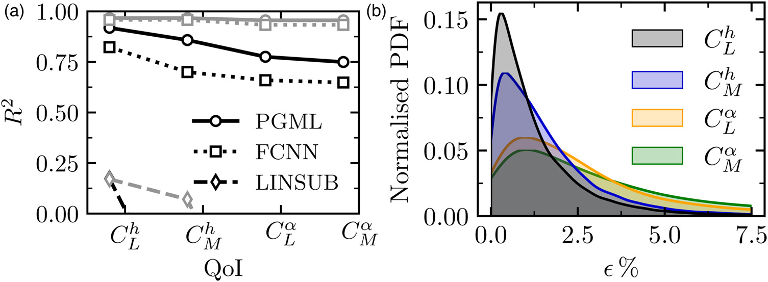
The error distribution of PGML on the validation set can be visualised as a probability density function (PDF). The relative error
Figure 2b reports the relative error distribution for each quantity of interest. For most of the validation samples, the relative errors are within
Figure 3.
Scatter plot of normalised QoI form validation set. The CFD and PGML predictions are on horizontal and vertical axis respectively. The QoIs are reported on each panel.
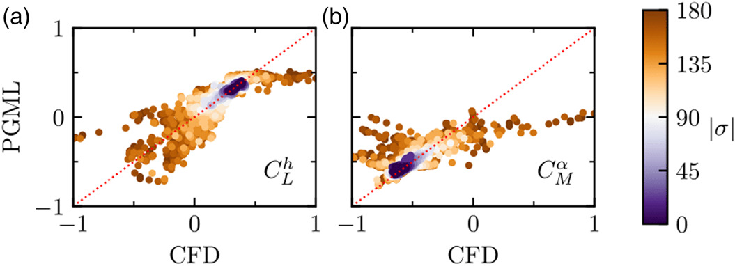
Although imperfect, the presented model fits its intended purpose: stall flutter occurs largely in the regimes where PGML performs well, i.e. flap modes, which are mostly plunge dominated, and at low interblade phase angles.
Prediction on unseen geometries
In this section, the selected machine learnt models will be examined more in depth and compared against the validation set results obtained with CFD. The validation set is composed of all the computations performed on the cascades obtained by varying the SC10 parameters one at a time. It is reiterated that, on the other hand, the training set is constituted of only SC10 computations, therefore all of the following results constitute an extrapolation in terms of geometry.
The plots in Figure 4 show the behaviour of plunge induced lift and pitch induced moment with increasing solidity. The steady state conditions,
Figure 4.
Predictions of plunge lift and pitch moment coefficients from CFD, PGML, FCNN and LINSUB against solidity. The steady state conditions are constant at M 1 = 0.85 β 1 = 3 ∘ k = 0.5 k = 0.7 k = 1.0 σ = 20 ∘
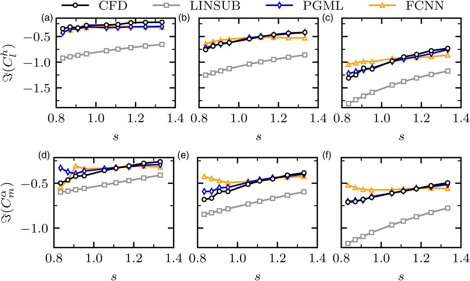
The FCNN produces results that are generally close to CFD and it is able to reproduce the behaviour with increasing solidity at low frequencies, although the agreement seems to degrade both as the frequency is increased and as the cascade operates at a solidity increasingly further from
On the other hand, the PGML model follows closely the FCNN at lower frequencies, but its predictions are visibly rectified by LINSUB at higher k, to the point that, in panels (c) and (f), the PGML predictions become parallel to those by LINSUB and overlap with the CFD almost perfectly, while the FCNN predicts a nearly constant behaviour. Furthermore, the slope of CFD and LINSUB predictions are nearly identical throughout the frequency range and are only offset by a value.
We now investigate a case with larger interblade phase angle. The plots in Figure 5 show the behaviour of plunge induced lift and pitch induced moment with increasing solidity. The steady state conditions,
Figure 5.
Predictions of plunge lift and pitch moment coefficients from CFD, PGML, FCNN and LINSUB against solidity. The steady state conditions are constant at M 1 = 0.85 β 1 = 3 ∘ k = 0.5 k = 0.7 k = 1.0 σ = 150 ∘
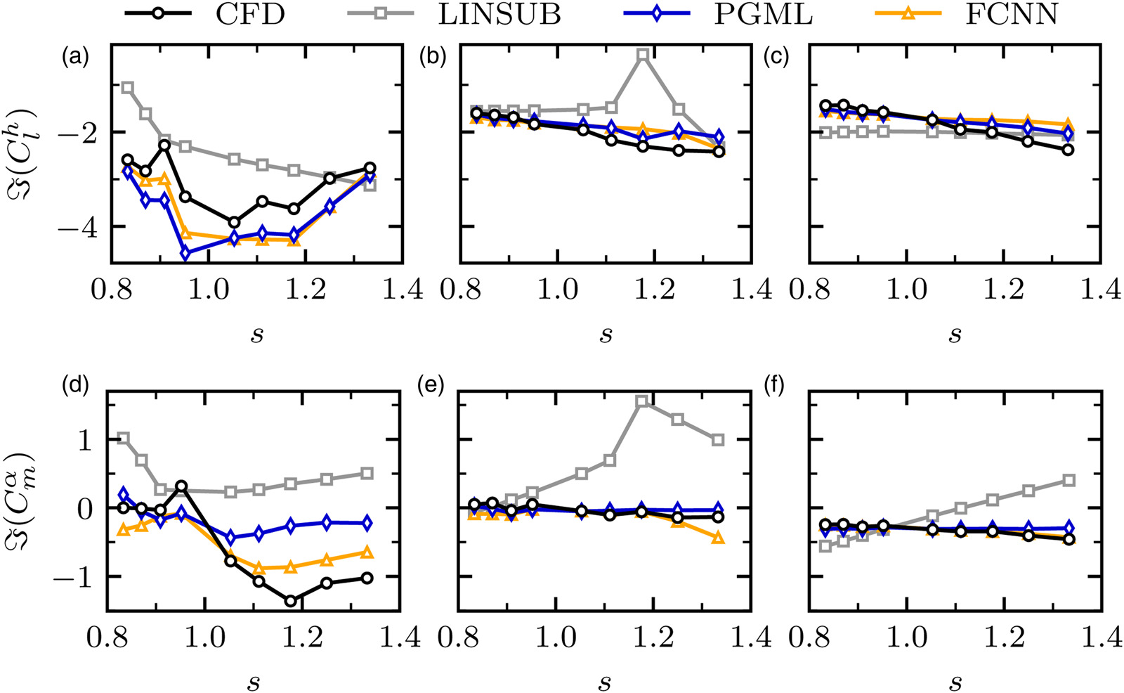
With
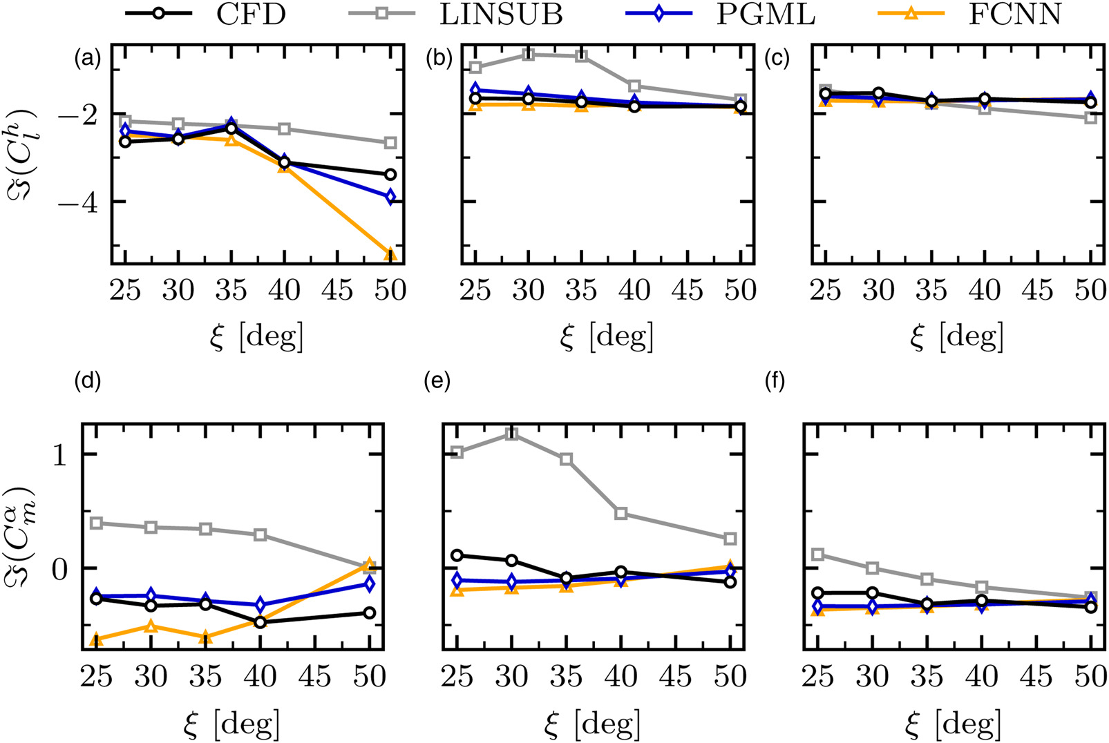
The plots in Figures 6 and 7 show the behaviour of plunge induced lift and pitch induced moment with increasing solidity with
Figure 6.
Predictions of plunge lift and pitch moment coefficients from CFD, PGML, FCNN and LINSUB against stagger angle. The steady state conditions are constant at M 1 = 0.85 β 1 = 3 ∘ k = 0.5 k = 0.7 k = 1.0 σ = 20 ∘
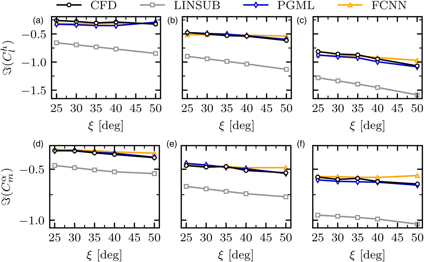
Figure 7.
Predictions of plunge lift and pitch moment coefficients from CFD, PGML, FCNN and LINSUB against stagger angle. The steady state conditions are constant at M 1 = 0.85 β 1 = 3 ∘ k = 0.5 k = 0.7 k = 1.0 σ = 150 ∘
Finally, a comparison of results obtained with a sweep in camber is shown in Figure 8. The steady and unsteady conditions are the same as the ones shown previously. Once again, the PGML is able to correctly predict the QoIs value across a range of conditions. We can appreciate only a small difference between the results from FCNN and PGML, and that is because the latter has learnt that LINSUB does not provide any significant guidance as the camber, and thus the loading, changes.
Figure 8.
Predictions of plunge lift and pitch moment coefficients from CFD, PGML, FCNN and LINSUB against camber. The steady state conditions are constant at M 1 = 0.85 β 1 = 3 ∘ k = 0.5 k = 0.7 k = 1.0 σ = 20 ∘
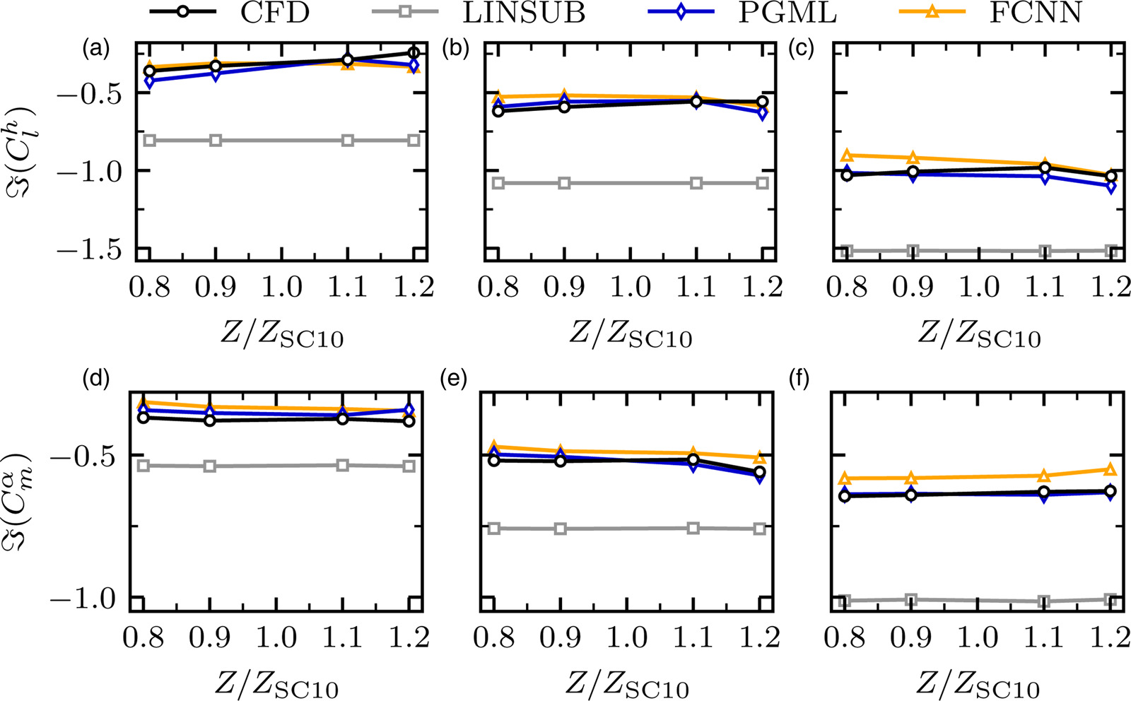
The input from LINSUB does not help capturing the change in camber, this makes intuitive sense as LINSUB is a flat plate model, though we can see that its effect is constant throughout the range, “pulling” the PGML predictions towards more negative values compared to the FCNN. The following conclusions can be drawn:
- the PGML relies largely on the physics guidance to produce predictions when a change of solidity or stagger angle is taking place, as their effect is modelled in LINSUB; on the other hand, the FCNN has to capture these effects solely through the steady state features provided, hence producing poorer results;
- the extent to which PGML relies on LINSUB depends on the combination of interblade phase angle and reduced frequency;
- the physics input has little contribution when a change in airfoil shape is taking place, as this effect is not modelled in LINSUB; nevertheless, it still provides useful guidance by rectifying the predictions, e.g. in Figure 8f we can see the PGML output being “corrected” towards more negative values.
Conclusions and future work
In this work, a physics guided neural network model has been presented.
The model leverages the PGML framework which is comprised of a fully connected neural network in which predictions of the QoIs from a reduced order model (ROM) are injected at some hidden layer. The ROM employed in this work is LINSUB, a semi-analytical method which models the aeroelastic response of a cascade of unloaded blades, accounting for important parameters such as cascade geometry and flow compressibility. The required data for model training was generated using CFD. The input features to the PGML are steady state quantities that are relevant for stall flutter and carry information regarding the cascade and blade geometry as well as blade loading. The unsteady input features are interblade phase angle and reduced frequency. The QoIs are four unsteady quantities, two lift and two moment coefficients, induced by two basic modeshapes: a plunge orthogonal to the chord line, and a pitch about the leading edge. In this way, the QoIs can be combined to predict aerodynamic damping for any flapwise bending modeshape. The current implementation of the PGML thus requires a steady CFD computation at prediction time to obtain the input features. Such an approach allows us to train the model on a reduced number of training samples as there is no need to pass the geometry directly as an input feature, which would require an unfeasible number of computations to build the training database.
The PGML is first trained with SC10 data only. The hyperpameters are tuned with a random search approach and the best model is selected with a 5-fold cross validation which, again, only employs SC10 data. Consequently, the model is tested on a large database of cascades and it is found that the PGML can predict the QoIs with good degree of accuracy, especially in the low interblade phase angle region, which is of most interest for stall flutter. It is also found that the prediction accuracy for plunge induced coefficients is higher than the pitch induced ones, due to the lack of an input feature pertaining to change in passage shape.
The authors are currently working on testing the model on cascade geometries resembling a tip section of a fan blade.