
Introduction
The usage of axial-centrifugal combined compressors is prevailing in small and medium aero-engines, including notable examples such as PWC’s PT6, GE’s T700, and Chinese WP11 engines. Centrifugal compressors are ideal for low flow rate applications due to their high single-stage pressure ratios, rotor stiffness, and simple structures. In addition, they exhibit superior efficiency level when compared to axial compressors at low flow rates. To increase the pressure ratio of modern compressors, the standard approach is to incorporate more stages. However, the multistage centrifugal compressors involve intricate flow path and pose challenges in maintaining high efficiency. Consequently, the number of centrifugal stages typically does not exceed two, which in turn restricts the pressure ratio of the compressor. To address this challenge, one solution is to incorporate several axial stages before the centrifugal stage, thereby leading to axial-centrifugal combined compressors. By doing so, a balance can be achieved between the high pressure ratio and high efficiency level.
Certain scholars have conducted research on axial-centrifugal combined compressors. Cousins (1997) studied the phenomena of stall and surge in several axial-centrifugal compressors experimentally, and evaluated a dynamic model that could capture the main features of stall and surge. Mansour et al. (2008) examined the performance of multiple RANS codes on a compressor which consists of a single stage axial followed by a single centrifugal stage. The results revealed that the k−ω/BSL turbulence model, incorporated in the CFX program, provided the most accurate predictions for the axial stage. Meanwhile, the k−ω/SST turbulence model, also implemented in the CFX program, was found to produce the best predictions for the centrifugal stage. Li et al. (2013) performed a numerical investigation on the flow with inlet circumferential distortion in two compressors: a combined compressor and its axial part alone. The primary distinction of the flow fields between the two cases was observed near the negative interface of distortion, where the orientation of the circumferential pressure gradient was opposite to the rotating direction. Zhao et al. (2013) simulated the flow with a clean inlet in the same combined compressor as Li et al. (2013), with a specific focus on the interactions between the rotors and stators. Their results indicated that the periods of unsteady pressure fluctuations on the stator surface were determined by the number of blades on both the upstream and downstream rotors, and the amplitudes of these fluctuations were influenced by the clocking effect of the rotors. Fu et al. (2021) used 14 million grids to conduct a full annulus numerical simulation on a combined compressor, comprising an axial stage, a centrifugal stage and a volute. They employed dynamic mode decomposition (DMD) to analyze the spike-type rotating stall of the compressor. As a result, two large low-frequency stall perturbations were captured, with the frequency approximately one-third and three-fourths of rotor frequency respectively. Despite the aforementioned papers, the majority of academic literature places greater emphasis on pure axial or centrifugal compressors, and, to the best of the authors’ knowledge, only a handful of publications have addressed the topic of combined compressors. Hence, further investigation is required to explore the flow characteristics of axial-centrifugal combined compressors, and the current study is motivated by the insufficiency of research on this topic.
This paper is structured as follows. Firstly, the examined compressor and the details of numerical settings will be presented. Subsequently, a comparison will be made between the compressor performance parameters obtained through experiments and CFD. Additionally, a three-dimensional flow fluid analysis will be performed. Lastly, conclusions will be drawn.
Methodology
The current study simulates the flows in an axial-centrifugal combined compressor, which was designed by Zhuzhou Liulingba Technology & Science Company in China (Li et al., 2023). The compressor consists of three axial stages and one centrifugal stage, as well as an inlet guide vane and an outlet guide vane. To provide a concise representation, the whole compressor is abbreviated as 3A1C in the current paper, while the individual blade rows are respectively referred to as S0, R1, S1, R2, S2, R3, S3, IMP, RD, and AD, as illustrated in Figure 1. Table 1 presents the parameters of the compressor. The impeller contains 15 main blades and 15 splitter blades.
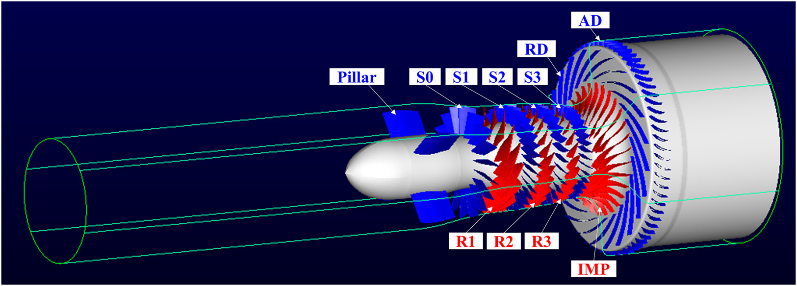
Table 1.
3A1C compressor parameters
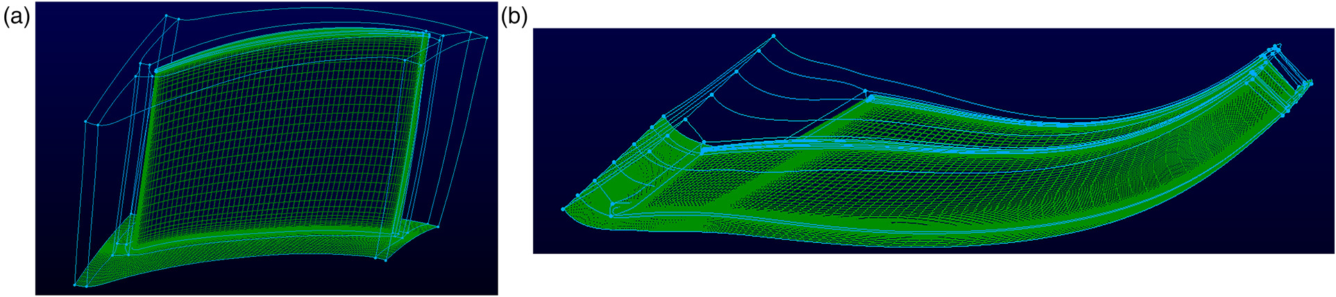
The computational domain used in this study encompasses the full annulus of the multistage compressor, as depicted in Figure 1. Structured grids are generated in each flow passage with NUMECA AutoGrid5, and a total of approximately 357 million cells are utilized. Table 2 lists the detailed distribution of grid points in each blade row. Considering the impeller is the most critical component for air compression, the grid cells in this region are refined. For the remaining blade rows, around one million cells are employed in a single passage, which is typically sufficient for conducting URANS simulations. The circumferential grid points are similar across each blade row since the sliding mesh method is employed at the rotor-stator interface. However, due to limitations in the grid topology, the number of circumferential cells at the impeller outlet is significantly larger than that in other regions. As examples, the grids for R2 and IMP are displayed in Figure 2.
Table 2.
Grid distribution
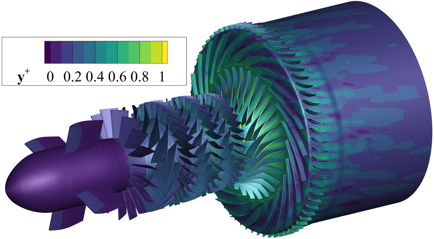
The simulation is performed with an in-house CFD solver. This solver has been previously verified in both axial and centrifugal compressors (Shi and Fu 2013; Jiang et al. 2021; Tian et al. 2021), and this paper presents its first application in an axial-centrifugal combined compressor. The solver is based on the compressible Navier-Stokes equation in the rotating reference frame and applies the cell-central finite volume formulation (Blazek, 2015). The inviscid fluxes are discretized with the rotated Roe scheme (Ren, 2003) with the third-order MUSCL reconstruction. The viscid fluxes are evaluated by the second-order central scheme. This study performs an unsteady RANS calculation, with 1,500 physical time steps included in one revolution period. For time integration, the solver employs the implicit lower–upper symmetric Gauss–Seidel (LU-SGS) scheme with sub-iterations in pseudo time, which provides second-order precision (Yoon and Jameson, 1988). The k−ω shear stress transport (SST) turbulence model (Menter, 1994) is used, and it is guaranteed that y+ is less than 1 on most solid walls, as shown in Figure 3.
The simulation of flows in rotors and stators is conducted in distinct reference frames: rotating and static, respectively. To accurately capture the interaction between rotors and stators, the sliding mesh method is adopted at their interfaces. Specifically, this method involves the linear interpolation of flow variables across the rotor-stator interface based on the transient physical angle of grid cells. At the inlet boundary, the total pressure and total temperature are given, and the flow is assumed purely axial. Turbulent kinetic energy and turbulent viscosity ratio are assigned as empirical parameters at the inlet for convenience. No-slip and adiabatic conditions are imposed on all solid walls. Two different outlet boundaries are implemented for different compressor operating points. For high mass flow rates, a uniform static pressure is enforced at the outlet of the computational domain. However, this can lead the simulation to diverge at low mass flow rates. To address this issue, an unsteady outlet pressure must be specified, and this study employs the throttle function (Cumpsty, 1989):
where Pout is the static pressure at the outlet, Patm = 101,325 Pa is the atmospheric pressure, and ˙mout is the mass flow rate at the outlet. Kt is a given coefficient which controls the throttle area. Different mass flow rates can be achieved by varying the throttle coefficient Kt.
Results and discussion
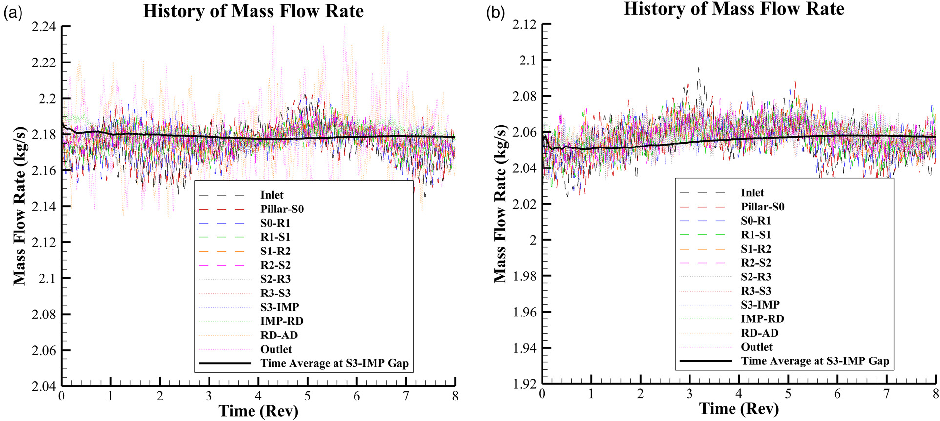
This study executes simulations at two distinct operating points of the compressor, namely the choked condition and the condition near peak efficiency. The convergence history of the mass flow rate for these conditions is illustrated in Figure 4. The dashed and dotted lines respectively depict the transient mass flow rates at twelve discrete cross sections, while the bold black line represents the time average value at the middle cross section between S3 and IMP. The simulations are deemed to have converged as evidenced by the stable fluctuation of all transient values around the average values. Particularly, the variations of the average values in each operating point are less than 0.5% over eight periods of revolution.
The actual performance parameters of the 3A1C compressor have been measured through experiments by Zhuzhou Liulingba Technology & Science Company. This paper presents a comparative analysis between the CFD and experimental results on the compressor performance map, as shown in Figure 5. The analysis reveals that the CFD-predicted choked mass flow rate (2.18 kg/s) is 2.2% lower than the experimental value (2.23 kg/s). Moreover, at the operating point near peak efficiency, the CFD predictions for the pressure ratio (3.37) and isentropic efficiency (0.726) exhibit a relative error of 4.0% and 4.6%, respectively, when compared with the experimental measurements of 3.51 and 0.761.
Figure 5.
3A1C Compressor Performance Map. (a) Total-total Pressure Ratio, and (b) Isentropic Efficiency.
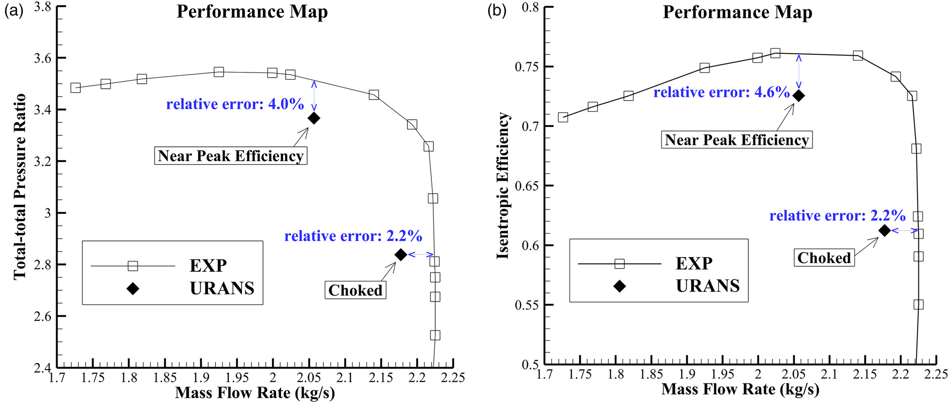
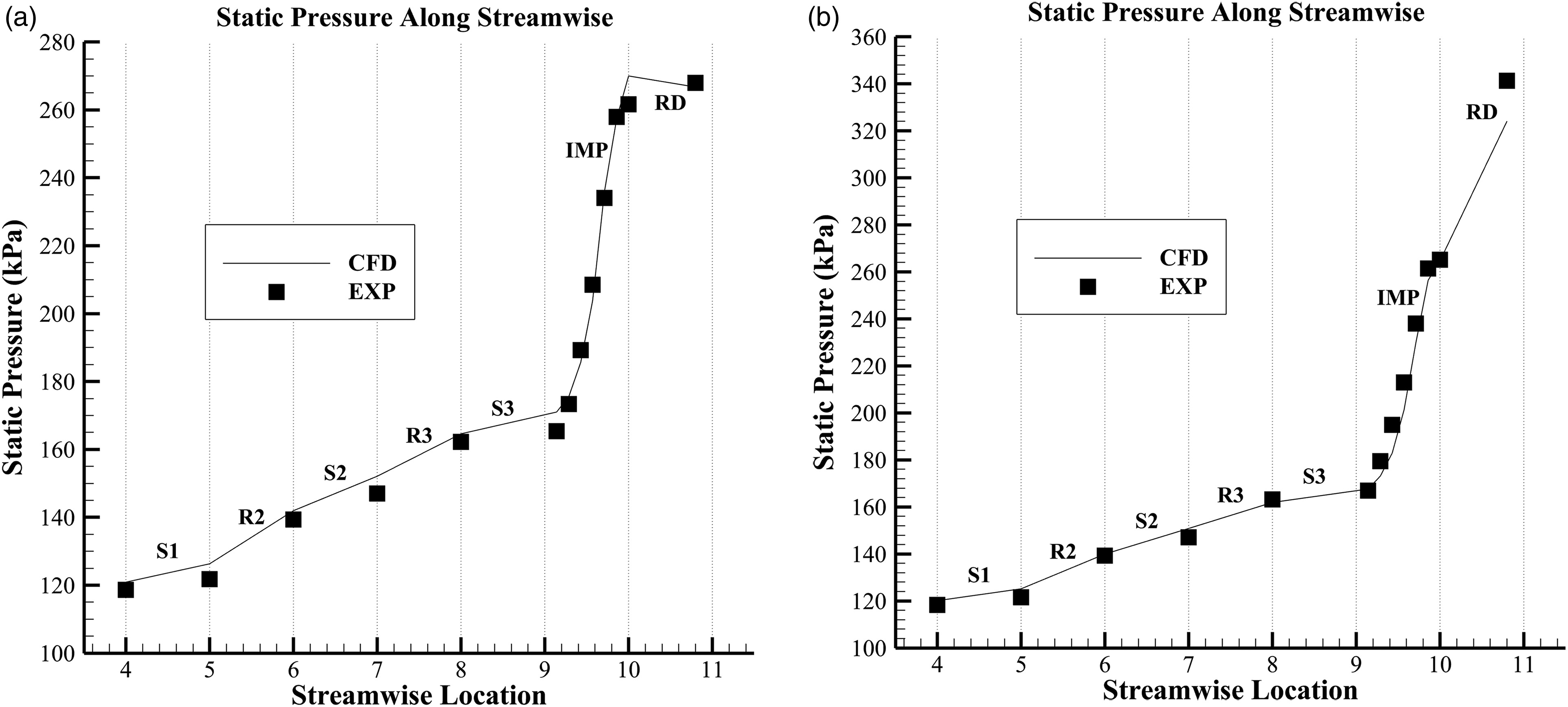
Figure 6 illustrates the static pressure at various streamwise locations, including both the CFD and experimental results. The abscissa in this figure indicates different streamwise locations, such as “streamwise location = 5” referring to the S1-R2 axial gap, and “streamwise location = 11” referring to the RD-AD gap. The experimental data are available from the inlet of S1 to the outlet of RD, which is the same range depicted in Figure 6. To ensure a fair comparison between the CFD and experimental data, the same mass flow rate is selected for the operating point near peak efficiency. However, when the flow is choked, the pressure ratio is held constant for comparison since the back pressure can vary without affecting the mass flow rate. As anticipated, the CFD results are in good agreement with the experimental data, especially in the axial stages and impeller. Nevertheless, at operating point near peak efficiency, the CFD-predicted static pressure at the outlet of RD is noticeably lower than the experimental result. This suggests that the CFD simulation underestimates the pressure rise in RD, which ultimately leads to a lower pressure ratio of the compressor as demonstrated in Figure 5a.
Figure 6.
Static Pressure at Different Streamwise Locations. (a) Choked, and (b) Near Peak Efficiency.
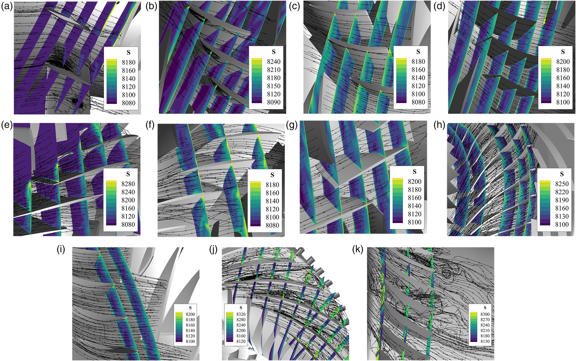
The following part of this paper is dedicated to examining the factors contributing to the choking of the 3A1C compressor. The overall flow field in the 3A1C compressor at choked operating point is displayed in Figures 7 and 8. In general, the flow maintains a smooth trajectory from the inlet until it exits the IMP, including the transitional region between the axial and centrifugal stages, i.e., S3-IMP gap. Despite the occurrence of some vortices, such as tip leakage vortices and separation on the suction surfaces, their effects are confined to a limited section of the flow passages. However, in the RD and AD regions, significant separation arises. Furthermore, the sonic surfaces, where the Mach number equals unity, occupy the throats of most flow passages within the RD, as is typical for choked flow. Conversely, sonic surfaces are scarce in other blade rows. These observations collectively affirm that the flow experiences choking in the RD.
Figure 7.
Overview of Flow Field in All Blade Rows at Choked Operating Point. (a) Vortices Indicated by Q Criterion, Colored by Pressure, and (b) Sonic Surface.
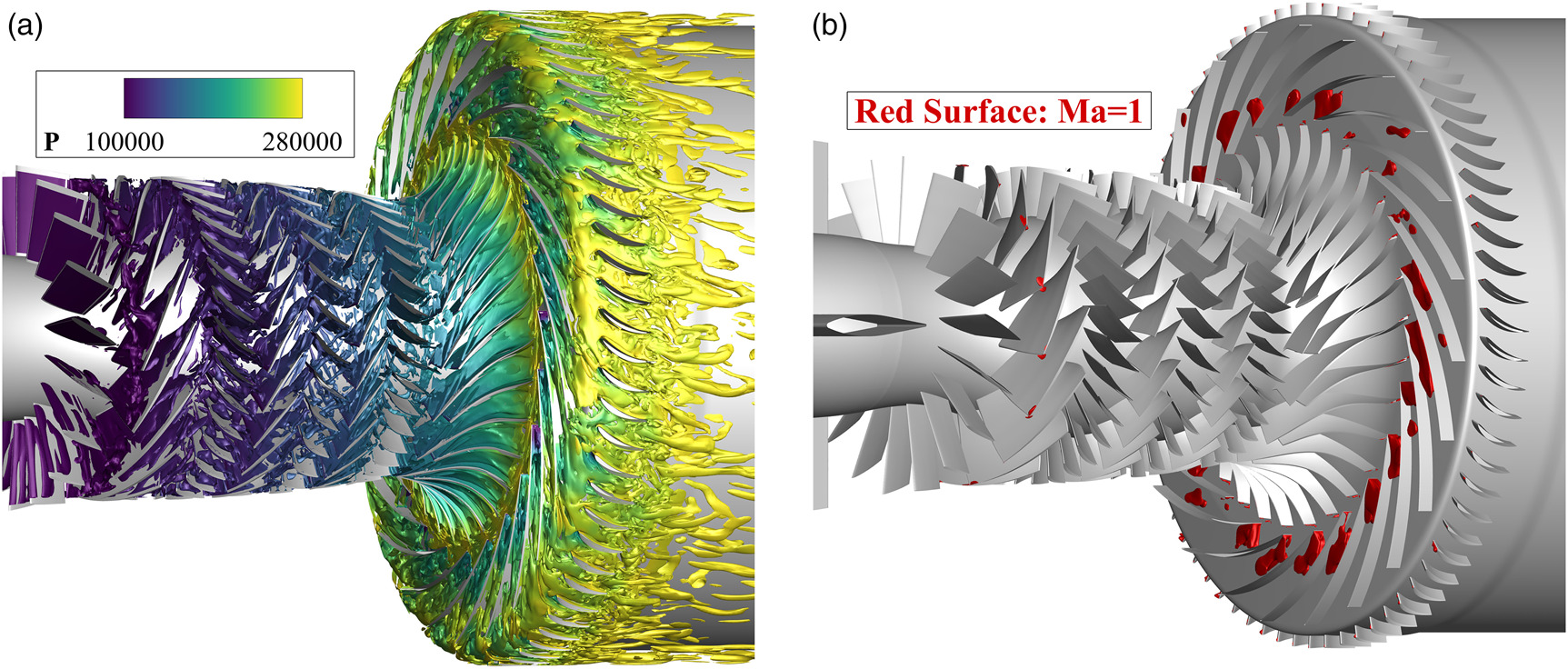
Figure 8.
Overview of Flow Field in Each Blade Row at Choked Operating Point, Colored by Entropy. (a) S0, (b) S1, (c) S2, (d) S3, (e) R1, (f) R2, (g) R3, (h) IMP, (i) S3-IMP Gap, (j) RD, and (k) AD.
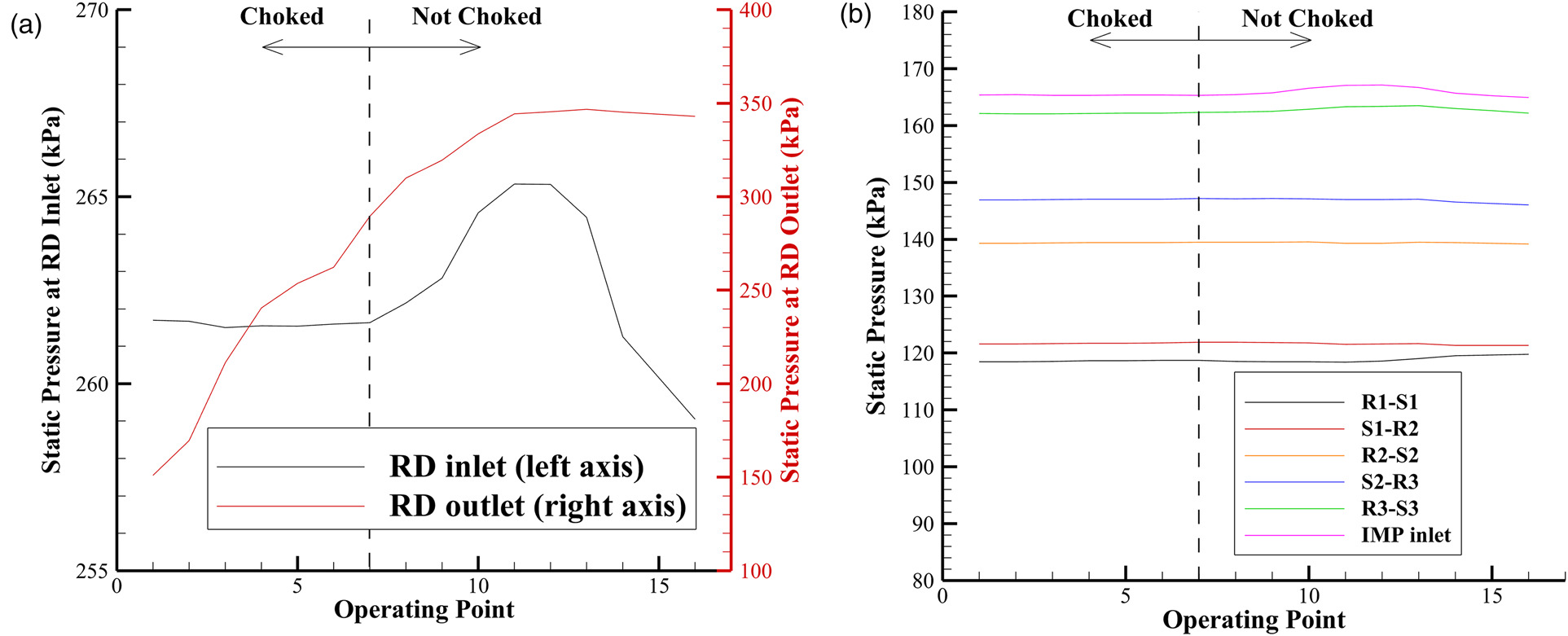
Additional evidence supporting this choked position is provided by the experiment. Figure 9 presents the experimental static pressure distribution at 16 operating points, ranging from choke to surge. The first seven operating points represent choked flow under different back pressure, while the remaining nine points operate without choking. Clearly, when the back pressure is altered at choked points, the pressure upstream the RD stays constant, while the pressure at the outlet of the RD varies. In contrast, at non-choked operating points, the pressure upstream the RD begins to change in response to the back pressure, which is particularly noticeable at the inlet of IMP.
Figure 9.
Experimental Static Pressure at Different Operating Points. (a) Inlet and Outlet of RD, and (b) Axial Stages and Inlet of IMP.
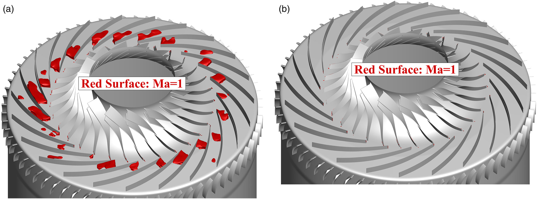
As is commonly observed, the choking phenomenon occurs when the flow velocity reaches sonic speed. This is distinctly demonstrated in Figure 10, which compares the sonic surfaces in the RD at the choked operating point and the near peak efficiency point. Specifically, at the choked point, the sonic surfaces obstruct the throats of most passages, whereas when the compressor operates near peak efficiency, the sonic surfaces dissipate.
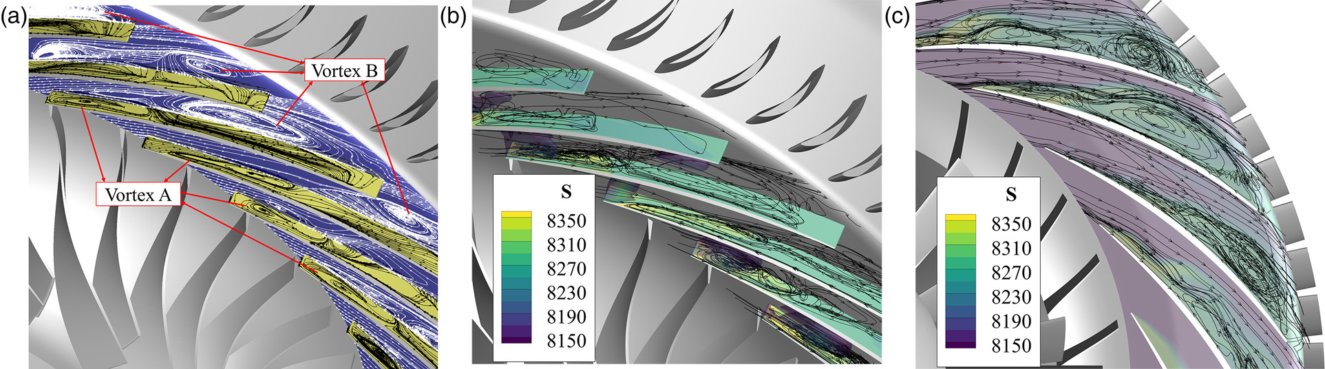
The flow within the RD exhibits circumferential non-uniformity and strong unsteady behavior. Despite this, the flow pattern is dominated by two prominent vortices, referred to as vortex A and vortex B, as depicted in Figure 11. In the figure, the yellow surfaces represent 3D surfaces around the blade, while the blue surfaces correspond to the isosurface of 20% blade height from hub to shroud. The axis of vortex A is nearly perpendicular to the blade suction surface, whereas the axis of vortex B is nearly aligned with the hub-to-shroud direction. These two vortices span the entire suction surface, occupying a significant portion of the passage, and are believed to be one of the underlying causes of choking.
Moreover, Figure 7a indicates that the tip vortices associated with R1 are predominantly localized within the upstream region of the rotor blades’ leading edge. This phenomenon is a common occurrence indicative of aerodynamic instability within axial rotors, signifying the possibility of an unstable flow regime within R1. However, it is noteworthy that as a whole, the 3A1C compressor is operating with maximal mass flow rate, denoted as “choked”, which is undoubtedly a stable operational state. This can be understandable as a consequence of the specific simulation conditions adopted in this study, wherein the rotational speed of the compressor is set at 70% of its design speed. At such reduced rotational speed, the fore stages of the compressor bear a large incidence angle, while the latter stages manifest a small incidence angle. This discrepancy in incidence angles underscores a noteworthy distinction between the multi-stage compressors and single-stage ones.
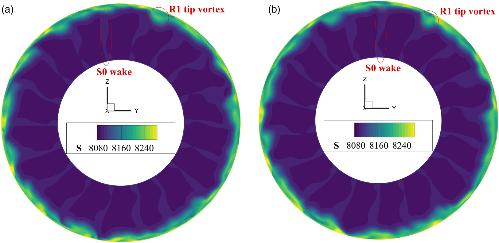
Further insight into the details of the R1 tip vortices is obtained through the utilization of three-dimensional flow structures, entropy contours at the R1 inlet cross-section, and frequency spectrum analyses, as depicted in Figures 12–14, respectively. Both Figures 12 and 13 are presented in the coordinate system fixed to the rotor. These two figures demonstrate the existence of multiple small, high-entropy fluid cells rotating relative to R1 blades. These cells exhibit irregularities in size and intensity, suggesting potential rotating instability in R1, caused by unsteady tip vortices. Figure 14 illustrates the power spectral density (PSD) of the pressure on the casing, encompassing both the CFD and experimental results. A discernible “hump” emerges within the frequency range situated below the R1 Blade Passing Frequency (BPF). This observation robustly bolsters the deduction that R1 is undergoing rotational instability (Day, 2016). Notably, some disparities manifest between the projected central frequency of this “hump” as predicted by CFD approach and the experimental results. These discrepancies could potentially be attributed to limitations of URANS, particularly the turbulence model.
Figure 12.
R1 Tip Vortices, Colored by Entropy. The Semitransparent Red Slice Refers to the Cross-section in Figure 13. (a) Time = 0 Rev, and (b) Time = 1/30 Rev.
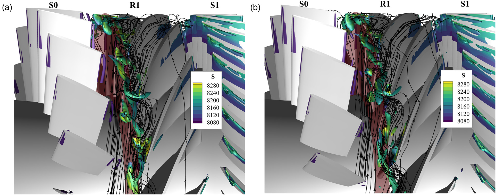
Figure 14.
Location of Pressure Probe, and PSD of Pressure on Casing at R1 Leading Edge. (a) Location of the Pressure Probe on Casing, and (b) PSD of Pressure on Casing at R1 Leading Edge.
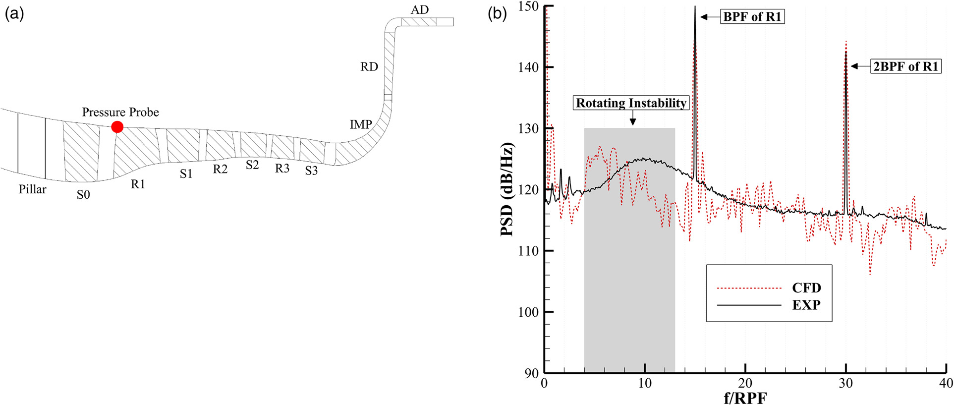
Figure 13.
Entropy Contours on R1 Inlet Cross-section, Located at the Semitransparent Red Slice in Figure 12. (a) Time = 0 Rev, and (b) Time = 1/30 Rev.
Conclusion
In this paper, a complete annulus URANS simulation of the 3A1C compressor is presented at two distinct operating points, choked and near peak efficiency. The main findings of the study are summarized as follows:
The compressor performance parameters at both operational points show good agreement with experimental results.
The occurrence of sonic surfaces at the throats of the flow passages causes the flow to choke in the RD, and variations in the back pressure have no effect on the pressure upstream of the RD when choked.
Two significant vortices primarily influence the flow within the RD at choked operating point, while the flow from the inlet to the outlet of the IMP remains relatively smooth.
Despite the compressor operating under choked conditions, the R1 tip vortices exhibit a characteristic of rotating instability, as evidenced by the presence of a discernible “hump” within the pressure frequency spectrum.
Nomenclature
URANS
unsteady Reynolds-Averaged Navier-Stokes
PWC
Pratt & Whitney Canada
GE
General Electric
k−ω/BSL turbulence model
k−ω/baseline turbulence model
k−ω/SST turbulence model
k−ω/shear stress transport turbulence model
DMD
dynamic mode decomposition
CFD
computational fluid dynamics
3A1C
three axial stages and one centrifugal stage
S0
the stator before the 1st rotor, i.e., the inlet guide vane
R1
the 1st axial rotor
S1
the 1st axial stator
R2
the 2nd axial rotor
S2
the 2nd axial stator
R3
the 3rd axial rotor
S3
the 3rd axial stator
IMP
the centrifugal impeller
RD
the radial diffuser
AD
the axial diffuser, i.e., the outlet guide vane
MUSCL
monotonic upstream-centered scheme for conservation laws
LU-SGS
lower–upper symmetric Gauss–Seidel
PSD
power spectral density
BPF
blade passing frequency
RPF
rotor passing frequency
y+
normalized first wall-normal grid space
Pout
static pressure at the outlet
Patm
atmospheric pressure, set as 101,325 Pa in this study
˙mout
mass flow rate at the outlet
Kt
throttle coefficient