
Introduction
Reduced order models (ROMs) are widely used to analyze the vibrations of rotors in turbomachinery. These are in particular beneficial when Monte-Carlo-Simulations to evaluate the impact of mistuning necessitate a large number of frequency response calculations. An overview of the mistuning phenomenon and model order reduction methods can be found in Castanier and Pierre (2006). After the ROMs were focused on a single stage at first, in the last two decades more and more methods were developed to deal with multistage rotors. Laxalde et al. (2007b) developed the multi stage cyclic symmetry method, where a modal analysis for the whole rotor is performed at once, but limited to a single harmonic. The complete ROM is then built from the modes of all harmonics. Therefore, some interstage coupling effects are omitted, but no substructuring with its inclusion of additional interface DOFs is necessary. Krattiger et al. (2019) give an overview of interface reduction methods for substructuring based ROMs. Sternchüss et al. (2009) use a superelement approach to reduce individual sectors of each stage before assembling them. Song et al. (2005) use the classical Craig-Bampton substructuring method to deal with multiple stages. Their main insights are to use travelling wave coordinates for each stage, thereby generating a single substructure for each harmonic of every stage and the reduction of the interfaces between stages. The interfaces are forced to be made up of concentric rings of nodes, which are reduced using Fourier basis functions. This reduction method was extended by Schwerdt et al. (2019) to include polynomial basis functions for the interface in addition to the Fourier basis, thereby reducing the number of necessary interface DOFs and eliminating the need for the nodes to have the same number of rings for both adjacent stages. The original and extended methods were applied to different problems, some of them including friction and aeroelastic effects (D’Souza et al., 2012; Battiato et al., 2018; Maroldt et al., 2022b).
The incorporation of aeroelastic effects into the ROMs is usually based on aeroelastic coefficients, aerodynamic stiffness, and damping, which are obtained by flutter calculations using the tuned system modes in traveling wave coordinates or blade-alone modes. Thus, an efficient calculation is possible, applying phase- or time-lagged periodic boundary conditions. Those models have been widely used to calculate tuned and mistuned responses of aerodynamically coupled structures. Aeroelastic coefficients can be calculated e.g. using linearized computational fluid dynamics (CFD) approaches and considered in structural ROMs, as done by Kielb et al. (2007) and Willeke et al. (2017). As shown by Kersken et al. (2012), comparing the results to conventional time domain simulations, and Meinzer and Seume (2020) comparing the results to experimental data, the linearized CFD models can give accurate results. Recently, nonlinear harmonic balance (HB) approaches have become increasingly important, as they are able to incorporate nonlinear aerodynamic effects, see e.g. Li et al. (2017). Another recent research area is the influence of multi-row interactions on the aeroelastic coupling coefficients. As e.g. shown by Schönenborn (2018), Maroldt et al. (2022a) and Gallardo et al. (2019) interactions with neighboring rows can significantly influence the aerodynamic work done on the vibrating blade.
When mistuning is present, the orthogonality of the eigenvectors regarding the nodal diameters is lost. This requires the calculation of aeroelastic coefficients for modes of all nodal diameters, even if the excitation is limited to one engine order. Consequently, the number of calculations needed increases rapidly. As described by He et al. (2007) this still holds for CMS approaches, as for an accurate prediction of the vibrational behaviour the aeroelastic calculation of constraint modes is needed in addition to the cantilever blade modes.
Only little work on ROMs for multi-stage turbomachinery, including aeroelastic coupling, has been reported in the open literature. Maroldt et al. (2022b) extended the model of Schwerdt et al. (2019) to include inter-stage aeroelastic coupling, showing that multi-stage excitation and inter-stage coupling can have a significant influence on vibration amplitudes and mistuning. The aeroelastic calculations were performed using a CFD nonlinear harmonic balance approach, which allows for multi-row coupling. The computational effort of the overall model reduction is mainly influenced by the calculation of the aeroelastic coupling coefficients, which were simulated for each DOF of the ROM. This leads to a high demand of computational resources. For the investigated
As mentioned above, neighboring rows can have a significant impact on the aeroelastic coefficients. Therefore, all rows or at least the neighboring rows in turbomachinery should be included in the model. The computational effort for a HB calculation of a whole compressor with IGV and s stages (or r rows) is then at least
Reduced order model
The reduction method presented in this paper is described in this chapter. Starting from the general equation of motion in the frequency domain
the following common assumptions are made: First, the matricesThe chapter is organized as follows: The multistage reduction method with a priori interface reduction is presented. It is extended using Characteristic Constraint Modes, and then methods to select the degrees of freedom of the reduced order model to include are discussed.
Multistage reduction model with a priori interface reduction
In this section the basic multistage reduced order model with a priori interface reduction from Schwerdt et al. (2019) is presented. It is an extension of the Fourier-Constraint-Modes method Laxalde et al. (2007a) and the basis for the improvements detailed in the next section. The method's main idea is to employ a Craig-Bampton reduction method with interface reduction, where each substructure is a single harmonic of one stage. Although it is later split up into the Fourier harmonics, for simplicity we will first consider the whole interface between adjacent stages. It is assumed, that this interface is ring shaped. The displacement of the interface degrees of freedom is described by a product of two families of basis functions. Polynomial basis functions are used in the radial direction, while a Fourier basis is used in the circumferential direction. As the displacement of the interface nodes must be described for each of the three cardinal directions (axial, radial and circumferential), if Fourier harmonics f from to
First, the stages are considered individually in cyclic coordinates. The DOFs of each stage
The interfaces are reduced using the basis vectors
All interface basis functions are distributed among the stage harmonics according to the equation
whereHere,
This reduction procedure is repeated for each harmonic of each stage. The substructures are assembled, prescribing displacement compatibility at the interfaces. After assembly the DOFs of the ROM are
The aeroelastic coefficients are calculated using the finished structural ROM, using the method described in Maroldt et al. (2022b) and discussed below in the section Aeroelastic Analysis. For each DOF of the ROM a flutter simulation is performed. The aeroelastic coefficients for this DOF are calculated using the resulting unsteady pressure distribution together with the displacement of all DOFs.
Characteristic constraint modes for multistage reduction
In this section the reduced order model is extended using the Characteristic Constraint Modes (CCM) method. The Characteristic Constraint Modes method is an interface reduction method originally developed to be used after a classic Craig-Bampton reduction Castanier et al. (2001) and Craig et al. (1968). Although applying it after the a priori interface reduction detailed above does not reduce the computational effort necessary to calculate the modes of the full rotor, this creates a more efficient reduced order model, while each DOF still represents monoharmonic displacements. If aeroelastic effects are to be included, this can reduce the number of CFD simulations necessary to achieve a given accuracy.
To achieve this goal, the CCM method is modified. Instead of calculating the characteristic constraint modes of all interface degrees of freedom, they are calculated for each interface harmonic
All DOFs of the whole rotor ROM can be grouped into inner DOFs and interface DOFs, ordered by the interface harmonic
(9)
To actually increase the efficiency of the ROM using CCM, not all characteristic constraint modes are kept in the reduced basis. Instead the least important CCM are dropped, which reduces the number of DOFs while decreasing the accuracy. But because the CCM capture the true interface displacements more efficiently, loosing the same amount of interface DOFs of the original ROM would decrease the accuracy even more. This is demonstrated in section Application.
Although not further analyzed in this paper, the relative efficiency of the CCM method rises with an increasing number of stages. If more stages are present, the CCMs can encompass multiple interfaces, with the opportunities for the CCM method to optimize the reduction basis improving with an increasing size of the CCM modal analyses (Equation 8).
DOF selection methods
To select which interface DOFs are the most important ones, two metrics are compared in this paper:
Both methods can be applied to both the original ROM as well as the ROM with characteristic constraint modes. They assign each DOF a score, that can be used to sort the DOFs from most to least important.The pseudo eigenfrequencies of the DOFs
The system eigenfrequencies method works by first selecting a number of system modes of interest, that the ROM should represent accurately. Then their eigenfrequencies are calculated using the ROM with all DOFs present. One by one, each DOF is removed from the ROM temporarily, and the eigenfrequencies of the modes of interest are calculated again. As is the case for all ROMs that project the system dynamics into a reduced subspace, the eigenfrequencies will rise with the removal of a DOF. The more the eigenfrequencies increase when omitting a specific DOF, the more important this DOF is for the ROM. In this paper the average relative eigenfrequency increase for all modes of interest is used, but other variants including weighting the modes of interest are possible. The relative increase of the eigenfrequency
Application
To analyze the reduction methods discussed above, they are applied to two rotors. The first rotor (Academic Rotor) is a simplified geometry without airfoils to show the structural dynamics and compare the effect of the different DOF sorting methods. Aeroelastic effects are incorporated into the analysis of the second rotor (Axial Compressor). Finally, the influence on eigenfrequencies DOF sorting method is applied to the a priori interface reduction to gain insight into the problem of optimally selecting the DOFs to include.
Academic rotor
The academic rotor consists of two stages with eight and five sectors respectively. The model has 8 821 and 14 037 nodes per sector for the first and second stage, quadratic hexaeder elements, and a total of about 400 000 DOFs when assembled. In Figure 1 the first stage is the flat bladed disk at the bottom, the second stage consists of the top bladed disk and the shaft. To compare the different interface reduction methods, the ROM consists of ten fixed interface modes per blade, totaling
Figure 1.
Characteristic Constraint Mode (Left) and its Two Main Constituents (Middle: 4ND, Constant Polynomial, Axial Displacement; Right: 4ND, Constant Polynomial, Radial Displacement).

When analyzing the characteristic constraint modes, most are dominated by one or a few of the original interface DOFs. This is expected as each CCM is limited to a single harmonic with 15 DOFs each. For rotors with more stages or more complicated interfaces requiring higher order polynomials, the CCM can be made up of more base DOFs each. Figure 1 show a CCM (left) which mostly consists of two base interface DOFs representing axial and radial displacement. Most notable is that for the CCM, there is less interface displacement for the same amount of blade displacement compared to the regular basis functions. This matches the goal of the CCM, to create DOFs which greatly influence the results, and other DOFs which can be ommited.
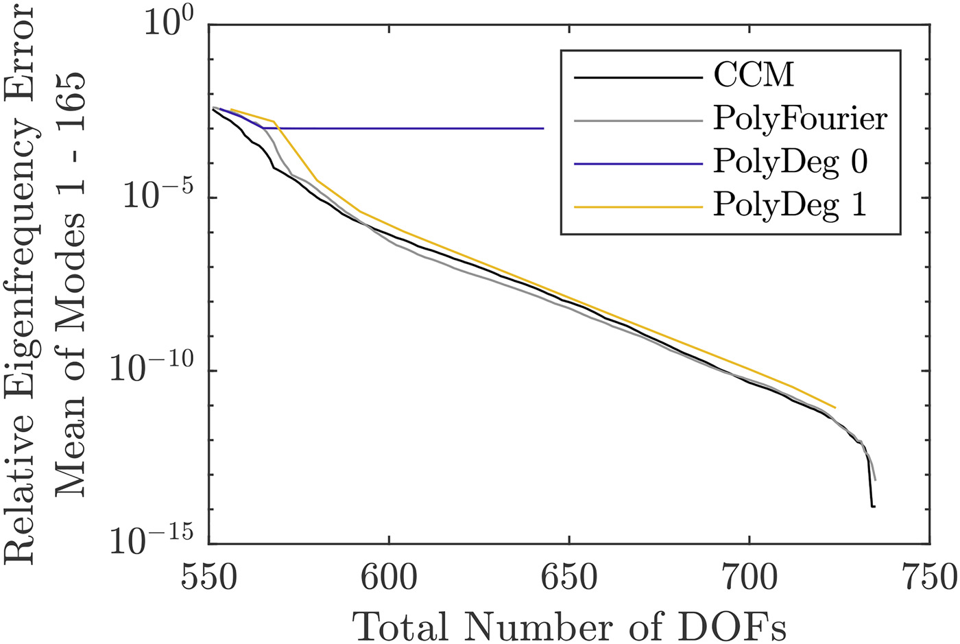
As a reference solution including aeroelastic effects is infeasible for the axial compressor, all comparisons will be made against the respective ROM with all DOFs present as a reference to keep a constant methodology throughout. The interface DOFs are then successively removed and the effect on the eigenfrequencies is shown in Figures 2 and 3. The colored lines represent the regular ROM without special sorting of the DOFs, where the polynomial degree is limited to zero to four respectively, and
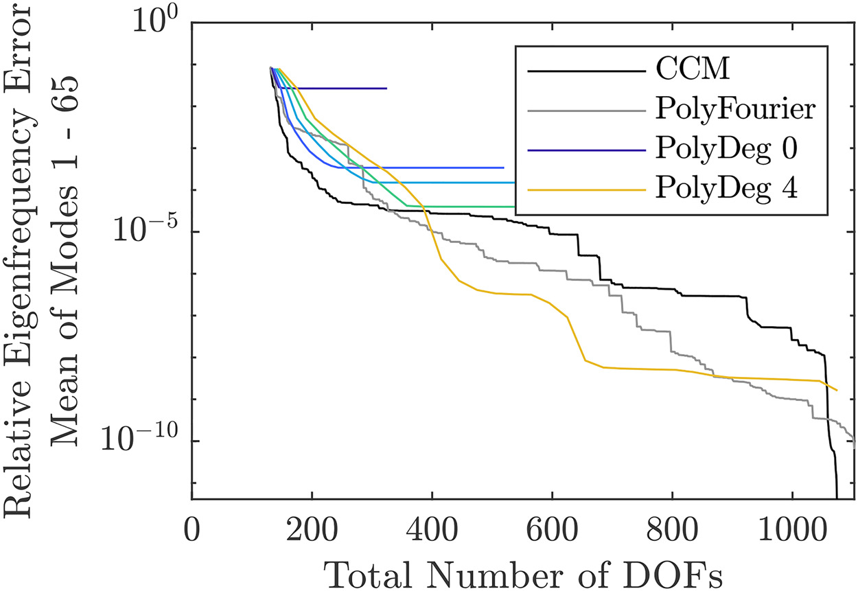
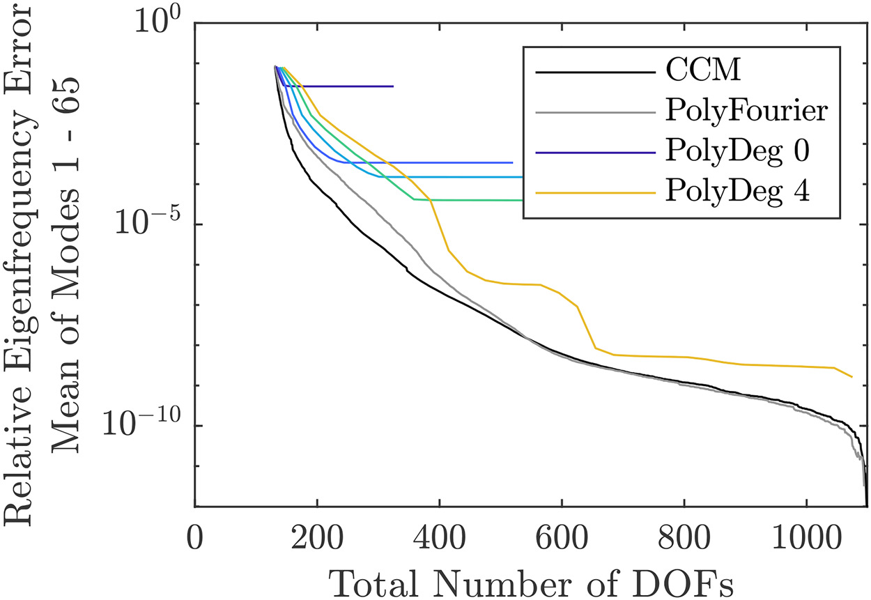
In black and grey, the errors are plotted when DOFs are removed according to the orders calculated by the DOF selection methods pseudoeigenfrequency of DOFs (Figure 2) and influence on system eigenfrequencies (Figure 3), where the regular DOFs are used for PolyFourier and the characteristic constraint modes are used for CCM. The pseudoeigenfrequecy sorting method is considerably worse, but, with the exception of ROMs with a large number of interface DOFs, still results in better ROMs than without any sorting method, especially if the characteristic constraint modes are used. Sorting the DOFs by their individual influence on the eigenfrequencies predictably results in consistently better ROMs, with the CCM method providing an additional benefit.
Axial compressor
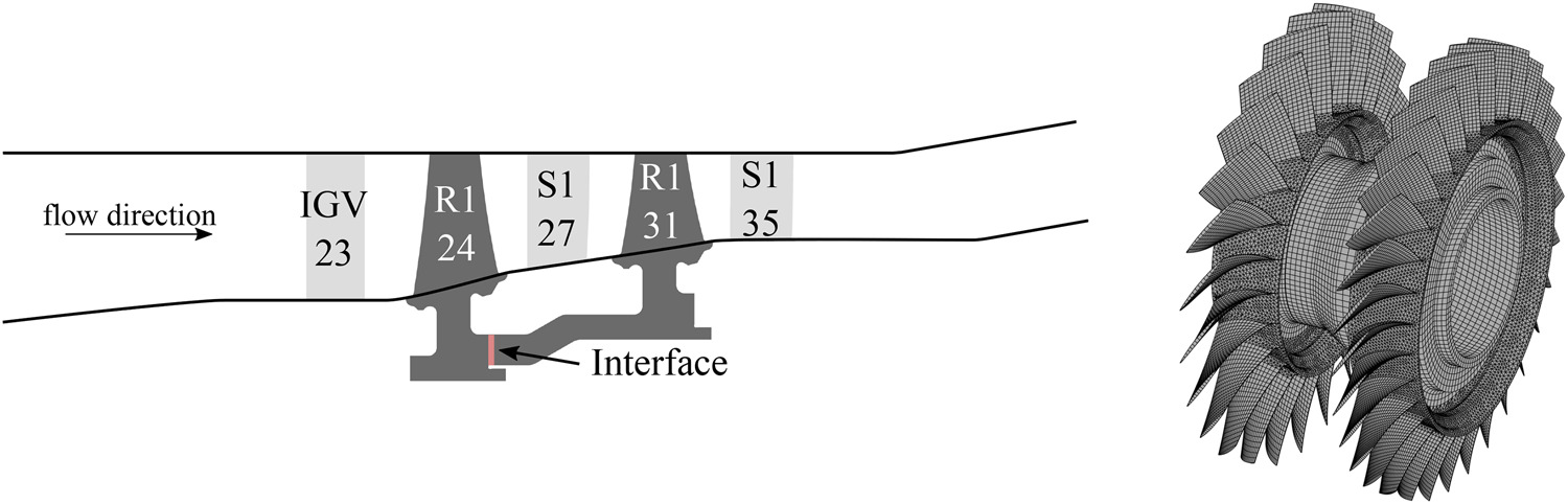
Figure 4 shows the axial compressor model used to evaluate the improved interface reduction method with aeroelastic coupling. The compressor rotor is made of Ti6Al4. The first rotor stage has 24 blades, the second one 31. To generate multistage coupled modes, the stiffness of the second stage was reduced to 65% of the nominal stiffness. The FEM model uses mostly quadratic hexahedral elements and has a total number of 1.96 million DOFs. For more details see Maroldt et al. (2022b).
The reduced order model uses 10 fixed interface modes per sector, for a total of
Aeroelastic analysis
Extensive flutter calculations are performed to calculate aeroelastic coupling coefficients of the DOFs. Aeroelastic simulations were only conducted for the
The aeroelastic coefficients are calculated via harmonic balance calculations (Frey et al., 2014) using the CFD code TRACE 9.3 by the German Aerospace Center (DLR). The harmonic balance simulations use the initial state solution of the whole
The flutter calculations use a reduced computational domain of only rotor 1, stator 1, and rotor 2. For each circumferential Fourier harmonic
Only the circumferential mode order of the Fourier harmonic
The unsteady pressure distributions on the blades created by the active DOF
Here, the aeroelastic coefficients are calculated for one rotational speed only. If accurate results for a broad speed range with multiple excited resonances are desired, the aeroelastic simulations must be repeated for different rotational speeds.
Results
First, the results of the ROMs without aeroelastic effects are analyzed. They are shown in Figures 5 and 6. For both ROMs, the maximum accuracy gain by sorting the DOFs is about a factor of ten, which is noticeably lower than the gain achievable for the academic rotor, where in the best case it is on the order of 100. One explanation for this might be the fact, that there are not enough Fourier harmonics to be included into the ROM, since
Figure 5.
Comparison of Interface Reduction Methods Without Aeroelastic Effects. Polynomial Degree Limited to Four. DOFs Sorted by the Omitted DOF Method.
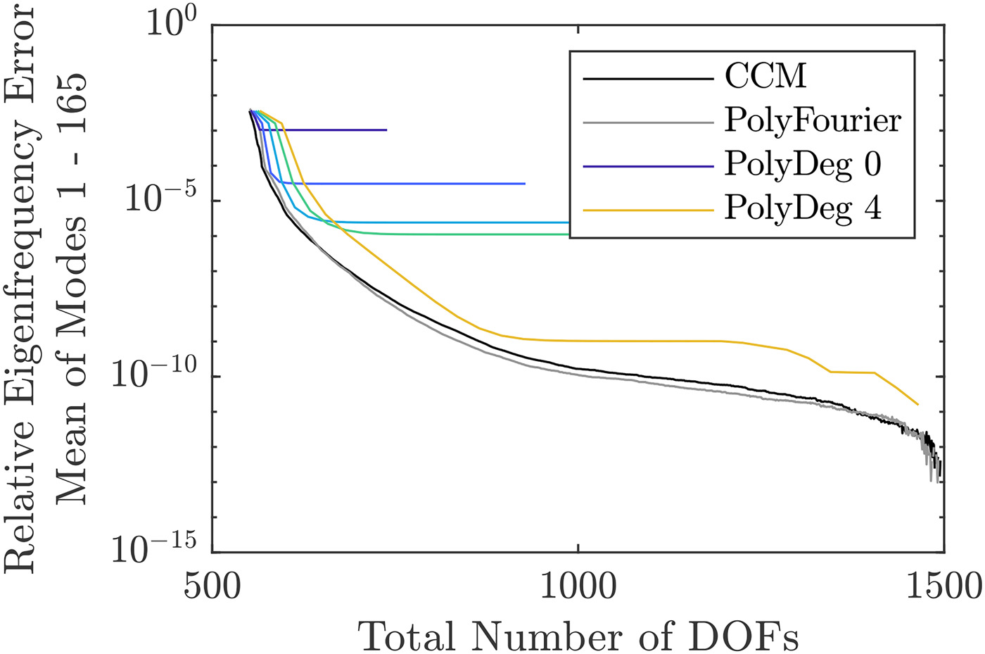
Figure 6.
Comparison of Interface Reduction Methods Without Aeroelastic Effects. Polynomial Degree Limited to One. DOFs Sorted by the Omitted DOF Method.
Adding aeroelastic coefficients, the system matrices cease to be Hermitian and the arbitrary damping must be considered. Therefore, the second order system of equations is converted to a first order system and the complex eigenvalues are analyzed. Their errors are plotted in Figures 7 and 8, split into absolute value and angle in the complex plane, to give an indication of the accuracy of the eigenfrequencies and damping values respectively. The number of DOFs refers to the second order system. The errors of the absolute value of the eigenvalues behave very similarly to the ROM without aeroelastic effects. This suggests that the aeroelastic effects do not significantly alter the mode shapes of the rotor. The errors of the eigenvalue angles are not given relative to the reference ROM, but as an absolute value because the range of aeroelastic damping values can include zero. Overall, the damping values are quite accurately captured by the ROM even with a low number of DOFs. Among the first 330 eigenvalues, the maximum and mean angle to the imaginary axis are
Figure 7.
Comparison of Interface Reduction Methods. Relative Error of the Absolute Value of the State Space Eigenvalues Including Aeroelastic Effects. DOFs Sorted by the Omitted DOF Method.
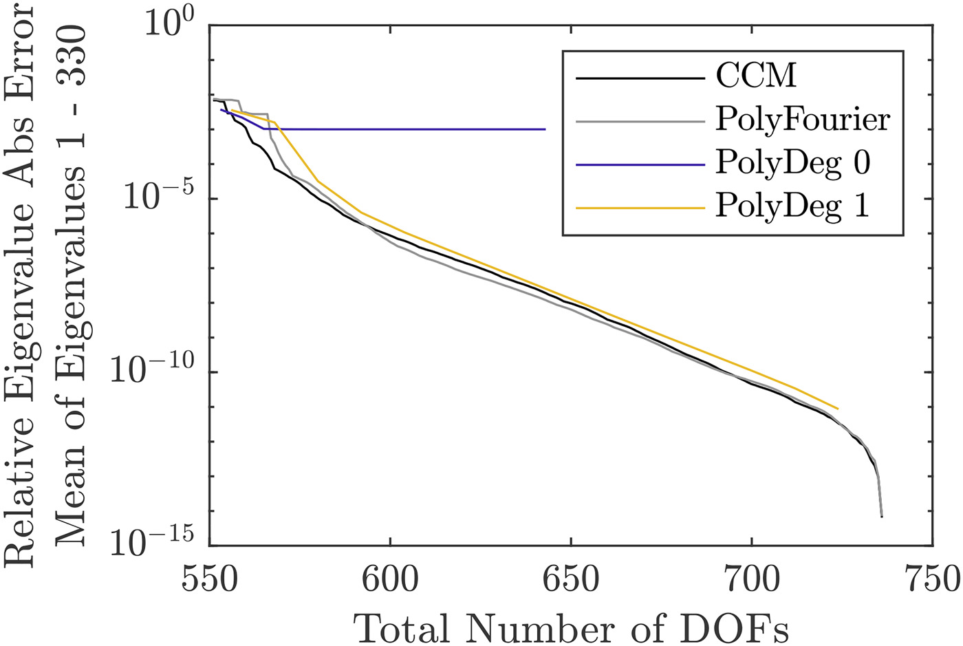
Figure 8.
Comparison of Interface Reduction Methods. Error of the Angle of the Complex State Space Eigenvalues Including Aeroelastic Effects. DOFs Sorted by the Omitted DOF Method.

Importance of interface DOFs
While the DOF selection methods outlined in this paper are helpful to increase the efficiency of reduced order models, they need a larger ROM in the first place from which DOFs are selectively removed. This is not an issue for a posteriori interface reduction methods, as in any case they require a larger initial reduction basis. To use a priori reduction methods most effectively, the DOFs to include must be selected in advance. To assess the relative importance of the interface DOFs with the combined Fourier- and polynomial basis functions, the order of the DOFs resulting from the influence on eigenfrequencies sorting method is analyzed in Figures 9, 10, 11 and 12. Here, the cumulative distribution of the interface DOFs is plotted from the most important to the least important DOF according to the sorting method. Figures 9 and 10 show the distribution of interface harmonics for the academic rotor and the axial compressor; the distribution of the DOFs grouped by polynomial degree is pictured in Figures 11 and 12. For both rotors, polynomials up to degree five were used, and interface harmonics up to degree
Figure 9.
Cumulative Distribution of the Interface Dofs Grouped by Nodal Diameter for the Academic Rotor. Sorted Using the Influence on Eigenfrequencies Method.
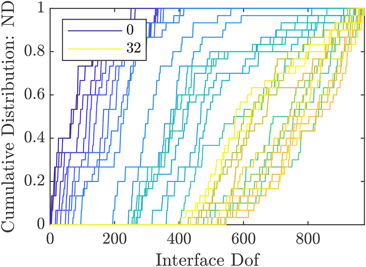
Figure 10.
Cumulative Distribution of the Interface Dofs Grouped by Nodal Diameter for the Axial Compressor. Sorted Using the Influence on Eigenfrequencies Method.
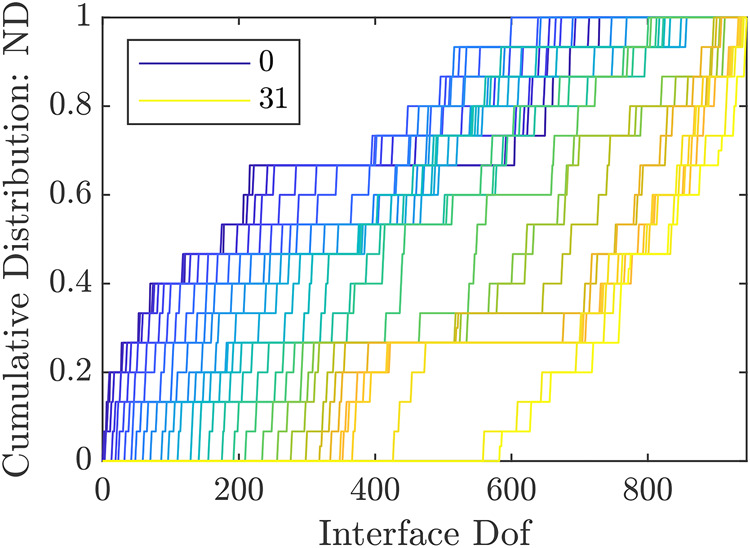
Figure 11.
Cumulative Distribution of the Interface Dofs Grouped by Polynomial Degree for the Academic Rotor. Sorted Using the Influence on Eigenfrequencies Method.
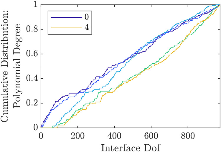
Figure 12.
Cumulative Distribution of the Interface Dofs Grouped by Polynomial Degree for the Axial Compressor. Sorted Using the Influence on Eigenfrequencies Method.
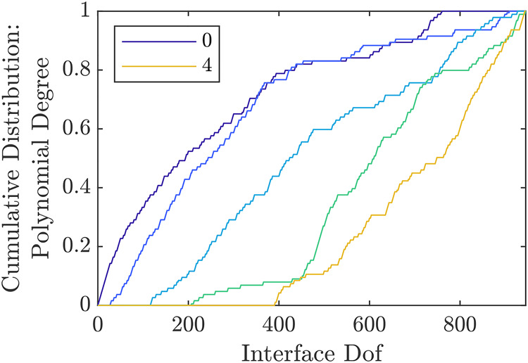
As expected, the lower harmonics and polynomial degrees are more important than the higher ones. This is easiest to see in Figure 12, where the most important DOFs all belong to the constant polynomial group. The higher order polynomials appear successively with increasing number of DOFs. Here, about 80% of constant and linear polynomial DOFs are more important than the first fourth order polynomial DOF. Comparing the plots of the two rotors, the academic rotor shows a greater spread in Fourier harmonic importance and a similar importance of the polynomial degrees, while the results are reversed for the axial compressor, which shows a greater spread of the polynomial degrees. This can be explained by the fact, that the academic rotor has fewer blades per stage compared to the axial compressor. Thus, to achieve a similar ratio of interface harmonics to the number of sectors per stage, more interface harmonics are needed for the axial compressor. Not pictured are the displacement directions. For both of the rotors, their importance is very similar, with axial and radial displacements being slightly more important than circumferential ones.
Going by these results, the following observations and recommendations can be made:
The constant and linear polynomial terms are almost equally important.
The maximum polynomial degree and interface harmonic to include must be balanced, not in absolute values, but relative to the number of sectors per stage.
The lower importance of the higher order polynomials demonstrates the advantage of polynomial basis functions compared to using only Fourier harmonics for each ring of nodes on the interfaces in the basic Fourier Constraint Modes method.
Equation 5 and Figure 1 show that the interfaces should be located in such a way as to minimize the influence of the interface DOFs. This is achieved by minimizing the interface displacements for all rotor system modes of interest. This way the system modes can be expressed well by the fixed interface modes alone. Conversely, the blade displacements of the Constraint Modes must be minimized. The choice of interface locations demonstrated herein is sub optimal, because its proximity to one stage means that the interface DOFs are required to accurately represent the system modes where this stage participates.
Conclusions
In this paper, a reduction method based on substructuring in cyclic coordinates for multistage turbomachinery rotors is presented. By including an a posteriori reduction of the interface between adjacent stages in addition to the a priori interface reduction used in other methods, less DOFs are needed for a given accuracy of the ROM. This enables the CFD simulations to be reduced in number, as fewer are necessary to capture aeroelastic effects for a given level of accuracy. Additionally, methods for sorting DOFs by their importance are compared, showing that ROM efficiency gains are achievable even without changing the ROM basis functions. Analyses of the resulting order of DOF provide insights that enable the user to better select of the interface basis functions for a priori interface reduction.
However, open questions and needs for further research remain. Instead of sorting the ROM DOFs with respect to their influence on the first n eigenfrequencies, one can use a weighted sum or select a subset of the eigenfrequencies, for example those close to a resonance crossing. In this case, the sorting method could also be extended to the fixed-interface modes, further reducing the number of CFD calculations.
Ideally, an alternative to the CCM method could be developed, thereby incorporating the goal to accurately represent some modes directly into the generation of the ROM instead of only using it later to sort the DOFs of a generally good reduction basis. Additionally, the method presented here must be compared to Laxalde's multistage cyclic symmetry method for different accuracy requirements and rotors of different sizes (numbers of stages). The development of a hybrid method is also possible, where multiple rotor sections consisting of multiple stages are connected using the interface reduction methods presented in this paper.