Comparison of non-premixed and premixed flamelets for ultra WET aero engine combustion conditions

The Water-Enhanced Turbofan (WET) is a future concept for aero engine applications being developed by MTU Aero Engines AG. Steam is injected into the combustion chamber to reduce temperature peaks and emission of pollutants. Depending on the steam content, the combustion process is modified. To analyze the effect of steam on the reaction kinetics and the temperature, detailed chemistry has to be employed. By comparing laminar flame speed and mole fraction distribution across the flame front, an appropriate chemical mechanism for the considered operating conditions including high steam loads was selected. Tabulated chemistry based on flamelets was employed, which enables the use of complex mechanisms in CFD analysis at reasonable computational costs. A comparison of premixed freely propagating flames and non-premixed counterflow diffusion flames to represent the manifolds was investigated. Various definitions of the progress variable are studied for ultra WET combustion considered under aero engine conditions. The manifolds from both model flames are compared from dry to ultra WET conditions with kerosene in an adapted Sandia Flame D large eddy simulation. While the premixed flamelets are generated efficiently, the results obtained with non-premixed flamelets are more reliable for the range of operating conditions investigated.

Introduction

One of the major optimization goals for the turbofan (TF) is the specific fuel consumption (SFC). In the last decades the SFC of the specific engine decreased based on the progression of single components. The benefits of the lower SFC on pollutant emissions was also a goal but not the main focus. During the last years the focal point changed. Furthermore, the regulations are limiting the future impact of aero engines on climate change. Based on the TF, MTU Aero Engines AG is developing the new Water-Enhanced Turbofan (WET) concept described by Schmitz et al. (2020). With the injection of high steam loads in the combustor, the enthalpy is increased and the peak temperature is decreased. The exhaust is cooled with a steam generator and the steam is liquefied through a condenser. The liquid water is separated, pressurized and passed through the steam generator and steam turbine before it is injected into the combustion chamber. Compared to a state-of-the-art aero engine, this concept potentially decreases NO_x emissions by 90% and contrails by 50%, as illustrated by Kaiser et al. (2022). The reduced SFC leads to lower CO₂. Therefore, the overall climate impact will be reduced by more than 40% (Kaiser et al., 2022). One component that is significantly influenced by the steam injection is the combustor. The direct injection of steam into the combustion chamber system majorly alters the combustion process. This has to be addressed in the early development phase already.

Numerical simulations are a cost-effective method for predicting combustion processes. This requires both a chemical mechanism and a combustion model. Chemical mechanisms of kerosene have been intensively researched over a wide range of operating conditions (Ranzi et al., 2005). The POLIMI mechanism for kerosene is provided by the CRECK modeling group of the Politecnico di Milano (POLIMI), which is considered detailed due to the number of species and reaction equations involved. Ranzi et al. (1995, 2005) have shown a wide range of inlet temperatures, pressures and equivalence ratios and compared it to different experimental sources. The laminar flame speed, ignition times and species production were investigated and the mechanism demonstrated a global agreement. The mechanism is valid for a large temperature range and well represents the formation of nitrogen oxides. The POLIMI can therefore be considered as a reference. Dagaut (2002) provided another detailed mechanism for heavy hydrocarbon fuels based on experimental data of a jet-stirred reactor (JSR). In a subsequent study, the mechanism was reduced and optimized for high pressure conditions using additional available experiments (Dagaut and Cathonnet, 2006). Due to the application for aero engine conditions with high pressures both mechanisms are included in this study. However, in many cases such a large number of species and reactions is not necessary or affordable for the considered application. For this reason, reduced mechanisms are established. Luche (2003) reduced the Dagaut mechanism (Dagaut, 2002) to a skeletal mechanism. This limits the applicability of the mechanism, but significantly reduces the computational cost. None of the available chemical mechanisms for kerosene combustion are particularly validated for ultra WET conditions. The high steam contents, however, have a significant influence on the chemistry as shown by previous researches Schimek et al. (2013), Göke (2012) and Hiestermann et al. (2022). Thus, based on the detailed POLIMI mechanism, the performance of the other mechanisms mentioned for the considered ultra WET condition is evaluated within this study.

The investigation of skeletal up to detailed mechanism necessitates the use of a combustion model that achieves tolerable computing times in industrial applications. Tabulated chemistry such as the flamelet-generated manifold (FGM) combustion model allows the use of complex chemical mechanisms at moderate computational cost, especially when compared with finite-rate chemistry (FRC) as shown by Yang et al. (2017) and Panchal et al. (2019). In contrast, FRC transports the species involved in the chemical mechanism and solves them directly in the simulation. This results in high accuracy at high computational cost, depending on the mechanism. However, this time advantage refers to only one of the three sub-aspects that are necessary for a numerical solution: Pre-processing, processing and post-processing. The pre-processing step of the FGM approach can be time intensive due to required tabulation of the chemistry. The thermo-chemical state is tabulated over the full range of independent variables by solving one-dimensional flames. The flamelets resulting from the one-dimensional flame describe the source term of the combustion and are therefore essential. Various configurations are conceivable: For premixed combustion, it is straightforward to use freely propagating or counterflow premixed flames. In aero engine applications, however, various technically premixed to swirl-stabilized diffusion flames are frequently used (Hassa, 2013). The present study addresses the question if it is beneficial to employ the significantly more challenging counterflow diffusion flame model for the tabulation (Ramaekers et al., 2005), especially for ultra WET conditions. Hansinger et al. (2017) compared freely propagating premixed and counterflow diffusion flamelets for a non-premixed application under atmospheric conditions with natural gas. Surprisingly, the results obtained with premixed flamelets were superior when compared to the experimental measurements. However, a comparison between premixed and non-premixed flamelets for aero engine and ultra WET conditions is not found in the literature. Moreover, separate investigations of both are rarely seen in detail. Furthermore, the general influence of steam on flamelets has not been investigated yet. The present study follows a approach similar to Hansinger et al. (2017), but for the entire range of dry to ultra WET aero engine conditions.

Regardless of the employed flame model, the generated manifolds depend on the progress variable and mixture fraction, which are both independent look-up variables. Ihme et al. (2012) summarized several definitions of the variable from different authors. Ma (2016), Ihme and Pitsch (2008) and Pitsch and Ihme (2005) carried out a parameter study for different progress variable definitions for natural gas at atmospheric conditions based on H₂O, CO, H₂ and CO₂. Fiorina et al. (2003, 2005a,b) proposed a general definition of the progress variable for dry combustion based on CO and CO₂. In the present study new definitions of progress variables, which are adapted to the considered ultra WET conditions, are compared to established definitions.

In order to verify the observations and results obtained previously, a CFD-FGM analysis is carried out. For this purpose, the Sandia Flame D is used with the original settings to validate the implemented combustion model and manifold approaches. The Sandia Flame D burner is a widely used experimental facility for validating numerical combustion models (Barlow and Frank, 1998; Schneider et al., 2003; Barlow et al., 2005). The experimental facility is designed to study turbulent combustion and jet flame break-up in a controlled laboratory environment and the effects of various factors such as turbulence intensity, equivalence ratio distribution, and chemical mechanisms on the combustion process. The main focus in this work is the analysis of ultra WET conditions. However, experimental results for ultra WET combustion with kerosene are not available in the literature, therefore the Sandia Flame D is adapted to the new operating conditions. The characteristic of the original Sandia Flame D and the dry aero engine simulation are compared. With the verification of the setup, influences such as jet break-up, axial velocity and temperature distribution are analyzed under dry and ultra WET conditions in FGM large eddy simulations (LES) with premixed and non-premixed look-up tables.

Chemical mechanism

A variety of chemical mechanisms for kerosene have been studied and validated. Especially in the last decades, the available experimental database has grown significantly (Dagaut and Cathonnet, 2006). Therefore, mechanisms have been optimized for various equivalence ratios, inlet temperatures and pressures. One of the most detailed mechanism is the POLIMI by the CRECK modeling group Ranzi et al. (2012, 2014, 2015) and Bagheri et al. (2020). Generated by the lumping procedures their mechanism includes specifications from low (LT) and high temperature (HT) oxidation, as well as the inclusion of NO_x and soot. The mechanism used here combines the variants except for the soot formation shown in Table 1. With 18250 reaction equations and 537 species the mechanism has been validated with experimental data from 0.08 bar laminar premixed flame up to 50 bar in a shock tube. The valid equivalence ratio range is from 0.5 to 2.0, but varies depending on the investigated pressure. The stiffness due to the amount of reaction equations leads to a great effort in solving a set of one-dimensional flames. It should be noted that the POLIMI is not optimized for oxidation under dilution with steam, but due to the high level of detail and the high number of reactions involving H₂O, it is used as the reference mechanism in the present study.

Table 1.

Chemical mechanisms for long-chain hydrocarbon fuel.

Chemical Mechanism	Fuel Species	Number of Species	Number of Reactions	Type
Luche^a	C₁₀H₂₂	91	694	Skeletal
Dagaut high pressure (Dag_HP)^b	C₁₀H₂₂	209	1,673	Detailed
Dagaut low pressure (Dag_LP)^c	C₁₀H₂₂	225	1,800	Detailed
POLIMI LT-HT-NOX (C1-C16)^d	C₁₀H₂₂	537	18,250	Detailed

[i] ^aLuche (2003).

[ii] ^bDagaut and Cathonnet (2006).

[iii] ^cDagaut (2002).

[iv] ^dRanzi et al. (2012, 2014, 2015).

One of the mechanisms being studied for influence under ultra high steam is established by Dagaut (2002). The original low pressure Dagaut mechanism (Dag_LP) has been validated for a equivalence ratio 0.5 to 2.0 under atmospheric conditions for kerosene. With a similar data set like the POLIMI the chemical mechanism is compared to experimental measurements of a JSR. The result is a reduced detail mechanism with 225 species listed in the Table 1. In order to close the gap between the detailed POLIMI and the Dagaut mechanism, a mechanism for high pressures was developed. The Dag_HP is based on the Dag_LP, but the optimization focus are pressures up to 40 bar. The comparison with the results of a JSR at 10 bar show some deviation, although a better agreement than the Dag_LP.

As the next gradation of chemical mechanisms the Luche (2003) is added to the study. As a skeletal mechanism the Luche includes fewer reaction equations and species shown in Table 1. At all there are three different version of the Luche mechanism available that only differ from the threshold on the flux of N species (Cerfacs, 2023). Independently of this, the three mechanism are valid for a equivalence ratio from 0.5 to 2.0 and pressures from 0.5 to 10 bar.

The analysis is divided into two sub-aspects i.e., the laminar flame speed and the mole fraction at constant adiabatic flame temperature for dry and wet conditions. Both are influenced by the reaction kinetics for each chemical mechanism. For an application in a real gas turbine, especially the laminar flame speed is essential. The laminar flame speed affects flame shape and is important for predicting flame stability. Therefore, the influence of steam depending on the mechanism is investigated. Another value in assessing the mechanism is the formation of intermediate and product species. The major species CO and CO₂ are therefore analyzed under ultra WET conditions.

Operating points

The challenging operating conditions in an aero engine combustion chamber have an influence on the analysis requirements. Both the long-chain hydrocarbon fuel kerosene and the high pressure are influencing factors. In addition, the inlet temperature is high, which increases the thermal loads in the combustion chamber. The WET concept addresses these issues by counteracting the thermal loads with the injection of significant amounts of steam. The considered operating points for dry to ultra WET conditions are defined in Table 2.

Table 2.

Operating conditions from dry to ultra WET.

p (bar)	T_in (K)	WGR (−)
20	600	0.0…0.3

They are representative for an aero engine according to the WET concept. The ultra WET combustion operating conditions are described using the water-gas ratio (WGR) in Equation (1), which defines the relationship between water and the sum of water and air. It is used here primarily to define the steam content at the inlet.

(1)

WGR=YH2O,uYH2O,u+Yair,u

Laminar flame speed

The laminar flame speed in Figure 1 is computed by solving a freely propagating one-dimensional premixed flame at a fixed adiabatic flame temperature of Tad=1800K. In that way, the influence of steam dilution on the reaction kinetics becomes apparent, which is otherwise masked by the dominant influence of the temperature. At constant equivalence ratio, the adiabatic flame temperature drops as the steam content increases due to the higher specific heat capacity and formation enthalpy shown in Figure 2. With the reduction of the temperature, the chemical equilibrium is shifted towards the products according to le Châtelier’s principle and exothermic reactions are favoured.

Figure 1.

Laminar flame speed vs. equivalence ratio WGR symbols: (+ WGR = 0.00), ( WGR = 0.10), ( WGR = 0.20), ( WGR = 0.30), chemical mechanism colors: ( Luche), ( Dag_HP), ( Dag_LP), ( POLIMI), T_ad= 1,800 K, T_in= 600 K, p = 20 bar.

https://journal.gpps.global/f/fulltexts/188264/JGPPS-00214-2023-01.01_min.jpg

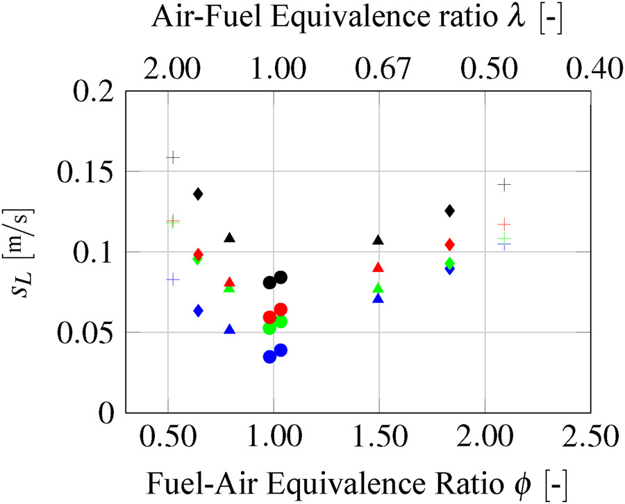
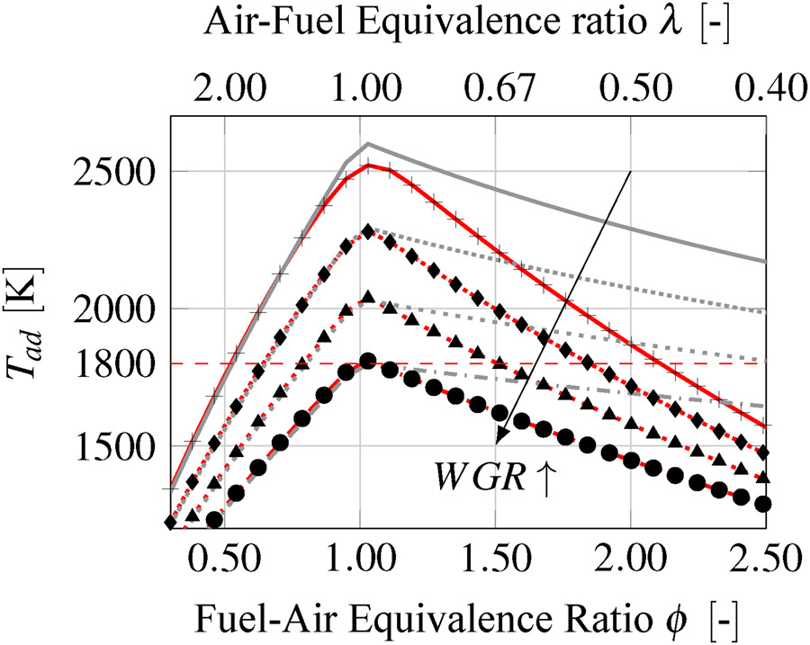
Figure 2.

Adiabatic flame temperature vs. equivalence ratio for (One-Step ), (Luche, Dag_LP and Dag_HP ) and (Polimi +) with WGR 0.0, 0.1, 0.2, 0.3 T_in = 600 K, p = 20 bar.

https://journal.gpps.global/f/fulltexts/188264/JGPPS-00214-2023-01.02_min.jpg

In the lean range, the relative discrepancy for the skeletal and detailed mechanisms related to the POLIMI is constant. Another observation is that the laminar flame speeds computed with the Luche mechanism are closer to the Dag_HP at high equivalence ratios. It is therefore understood that at a constant flame temperature, the laminar speed decreases in the lean region and increases in the rich region. Thus, the steam changes the local conditions of the flame. Especially if the results are compared with dry conditions (Wu et al., 2018). A direct comparison of the Dag_LP with the Dag_HP provides a result that was not to be expected. In terms of laminar flame speed, the optimized Dag_HP for high pressure applications exhibits greater discrepancies with the POLIMI than the Dag_LP.

Concentration of carbon monoxide and dioxide

Figure 3 shows the mole fraction of the dissociation of CO and CO₂ across the flame front. Generally speaking, the temperature reduction caused by steam addition promotes the exothermic CO₂ production. To eliminate this dominant effect, the molar fractions are analyzed at constant adiabatic temperature for the dry and ultra wet conditions in the rich region.

Figure 3.

Mole fraction vs. normalized length of CO () and CO₂ (), chemical mechanism colors: ( Luche), ( Dag_HP), ( Dag_LP), ( POLIMI), T_ad= 1,800 K, T_in = 600 K, p = 20 bar. (a) Dry combustion WGR = 0.00 at ϕ = 2.09. (b) Ultra WET combustion WGR = 0.30 at ϕ = 1.03.

https://journal.gpps.global/f/fulltexts/188264/JGPPS-00214-2023-01.03_min.jpg

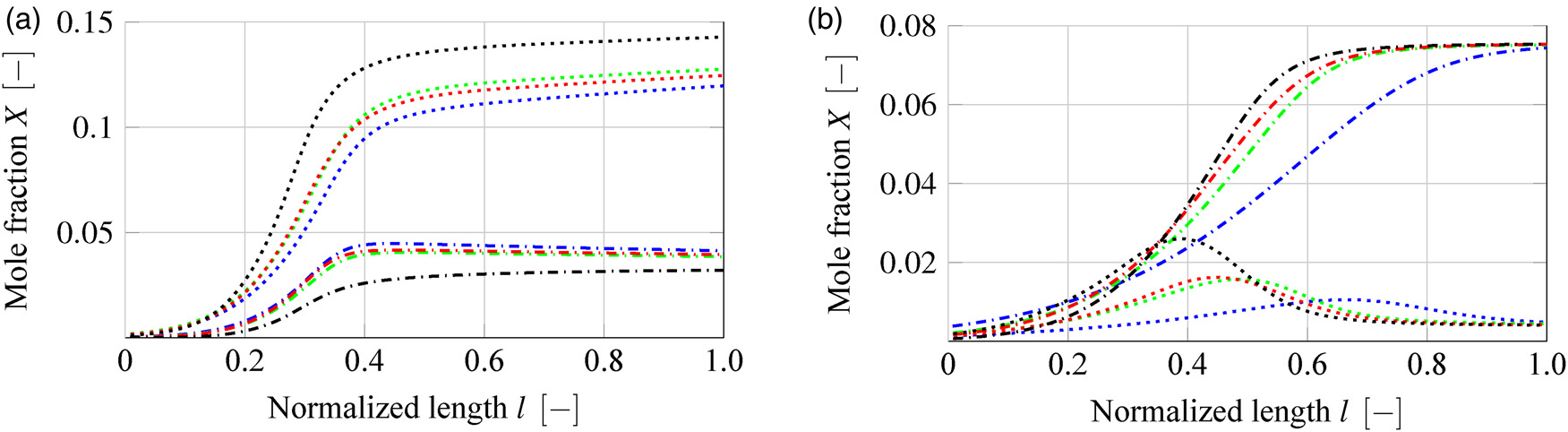
In Figure 3(a) the profile of CO₂ from POLIMI differs and is lower compared to the others. With less complexity in the mechanism, the local CO₂ production of the other mechanisms is overestimated. The opposite is shown for CO. The Dag_HP shows a slightly better agreement for both mole fractions. Differences in the distribution exist especially for CO under ultra WET conditions, see Figure 3(b). This behavior is based on the steam injection and the almost stoichiometric equivalence ratio. With a lower ratio of O₂ to C the production of carbon monoxides and dioxides is less independent of the mechanism. However, under dry conditions, CO production should dominate over CO₂ even with the same equivalence ratios. Therefore, the shift in the order of production rates is due to the effect of H₂O on the reaction kinetics. The wet conditions additionally lead to a change in the preferred mechanism to Dag_LP. The Luche mechanism shows significantly greater deviation in WET combustion.

In conclusion, for the present operating points, the Dag_LP best matches the laminar flame speeds and mole fraction profiles at ultra WET aero engine conditions obtained with the POLIMI. As the latter is considered to be too time-consuming in the pre-processing step for industrial applications, the Dag_LP is used in the following. The other mechanisms are not explored further in the present investigation. The reason for this is that since the chemistry is based on table generation of the flamelets, it can be assumed that similar behavior is expected in the three-dimensional simulation.

Flame configuration

The flamelet assumption describes a turbulent flame as an agglomeration of thin, locally one dimensional, laminar flame elements (Peters, 1984, 1988; Peters and Kee, 1987). This assumption is the basis for a variety of flame models. A comparison between the non-premixed and premixed flames is made using two types of model flames, see Figure 4. The freely propagating flame is a simplified approach to generate the flamelet database. In contrast, the non-premixed counterflow diffusion flame is significantly more complex and time-consuming in the pre-processing step. The one-dimensional premixed flame is simulated with a freely propagating flame, where a perfect mixture of oxidizer, fuel and additional steam is provided at the inlet on the left side in Figure 4(a). The velocity at the inlet is equal to the laminar flame speed in order that the flame front position remains fixed.

Figure 4.

Flame configurations. (a) Freely propagating flame. (b) Counterflow diffusion flame.

https://journal.gpps.global/f/fulltexts/188264/JGPPS-00214-2023-01.04_min.jpg

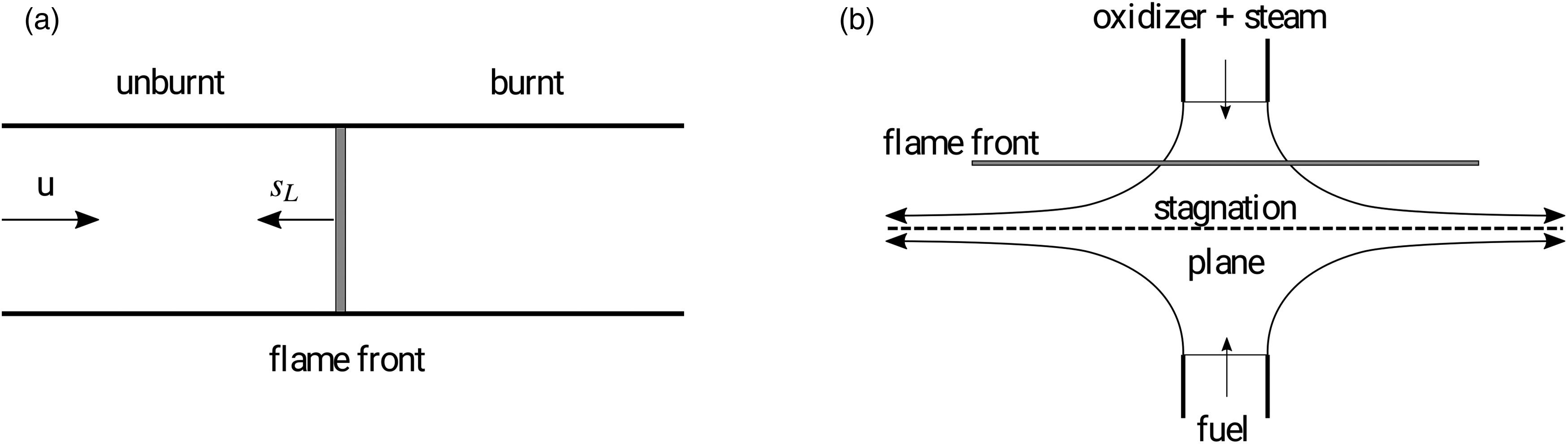
The inlets of the counterflow diffusion flame are divided into fuel and oxidizer with additional steam, as shown in Figure 4(a). The steam is added to the oxidizer stream only. The two separate streams form a stagnation plane. The flame stabilizes between the stagnation point and the oxidizer inlet based on the inlet fluxes. Contrary to the premixed configuration, the entire range of possible mixture fractions is found within the domain.

In order to solve the equations for both flames a combination of Cantera (Goodwin et al., 2022) and the open source code Ember (Speth, 2022) is implemented in the pre-processing program with custom modifications. Therefore, a switch between a steady-state Cantera and unsteady simulation Ember can be automatically conducted with user defined functions.

Flamelet table variables

The mixture fraction and the normalized progress variable are the two independent variables that describe the flamelets. The mixture fraction is formulated according to Bilger (1980a,b, 1989). The Bilger coefficient β in Equation (2) characterizes the current mixture at position x or cell i.

(2)

β=1m∑knC,kYkWk+1n∑knH,kYkWk−1m+(n/4)∑knO,kYkWk

The value nk represent the number of atoms of the respective species. The coefficients m and n are defined by the number of C and H atoms in the hydrocarbon fuel C_mH_n. In this definition carbon C, hydrogen H and oxygen O are used. The mixture fraction is defined as

(3)

Z=β(comp)−β(ox)β(fuel)−β(ox),

where β(ox/fuel) is the Bilger coefficient at the oxidizer and fuel side. Z=0 for pure oxidizer and Z=1 for pure fuel.

The second independent variable is called normalized progress variable. For this purpose, the progress variable is introduced first. In order that the progress of the combustion can be defined, the progress variable YC is of significant importance for the manifolds. The manifolds in a premixed flames are only defined by the YC. In general YC is defined as the sum of mass fraction k divided by the molar mass in Equation (4).

(4)

YC=∑kYkWk

The progress variable is based on the definition of Ma (2016) with weighting factors w and the mass fractions Y of water, carbon dioxide, hydrogen and carbon monoxide defined in Equation (5).

(5)

YC=wH2OYH2OWH2O+wCO2YCO2WCO2+wH2YH2WH2+wCOYCOWCO

A direct comparison and a simple application in the numerical solver is facilitated by normalizing the progress variable C. Above all, the direct comparison of different variables is possible. The manilds are used as evaluation criterion with C.

(6)

C=YC(Z)−YC,min(Z)YC,max(Z)−YC,min(Z)

The determination of the weighting factors w and the species considered depends mainly on the fuel and the operating conditions. It is necessary to verify which definition describes the manifolds in an optimal manner.

Premixed: freely propagating flame

If the premixed flames are compared with the non-premixed flames, the difference becomes apparent as soon as the flamelets are created. One-dimensional premixed flames describe the changes of the thermo-chemical state of a perfectly premixed gas depending on the axial position x until complete combustion of the mixture. For each freely propagating flame in Figure 4(a), the mixture fraction at the inlet is fixed. Thus the entire C−Z-space has to be represented by multiple premixed flames. Representative examples of single flames are illustrated as dashed lines in the Figure 5(a).

Figure 5.

Temperature vs. mixture fraction of premixed freely propagating flame and counterflow diffusion flame with normalized progress variable isolines. (a) Freely propagating flames. (b) Counterflow diffusion flames for steady and unsteady branches.

https://journal.gpps.global/f/fulltexts/188264/JGPPS-00214-2023-01.05_min.jpg

The lean and rich flammability limits of a premixed flame limit the available Z range. In the present study mixture fractions in the range 0.03 to 0.1785 are simulated as shown in Figure 5(a). The area remaining below the lowest mixture fraction and above the highest (gray) is interpolated, since the values on the left and right side of the C−Z-diagram correspond to pure oxidizer or pure fuel, respectively. This assumption is legitimate if the region occurs rarely and the influence on the combustion is small. Accordingly, with this method it is possible to cover the entire C−Z-space.

Non-premixed: counterflow diffusion flame

A one-dimensional counterflow diffusion flame describes a single non-premixed flamelet at a specific strain rate. In contrast to the premixed flame, a single flame covers the entire mixture fraction range. However, for the description of the whole C–Z space a single flamelet is not sufficient. To simulate further flamelets, the method of strain rate increase is applied. The flame is quenched at the higher strain rate until the flame is extinguished due to the high velocities. This is illustrated by various normalized progress variable isolines in Figure 5(b).

The simulation of the whole C–Z space is separated in two parts. In the steady state approach the flamelets are calculated beginning from a strain rate a=0 (equal to equilibrium conditions) until the flame extinguishes. The so-called stable branch describes the area of the flame where it can be assumed stable (Pitsch and Ihme, 2005). From this point on, the time-independent simulation does not provide any further solutions and neglected the unstable flames. For the unstable branch, the equations in Appendix A are solved in time from the region of the last stable flamelet of the steady state simulation up to the theoretical extinction of the flame. The result is a complete representation of the possible C over Z space.

Progress variable study

Progress variable requirements

The definition of the progress variable is not unique but the choice is based on some principles proposed by Ihme et al. (2012). The definition of C should result in a reasonable transport equation. This transport equation is used in the numerical simulation with the FGM model to solve the combustion. The included reactive species should represent the combustion process in comparable time scales. Moreover, the description of C and Z represents the thermodynamic and chemical space. Therefore, the involved parameters should represent the entire framework. Also is it necessary that the parameters are independent for the definition of the manifolds. More details are shown in the publication of Ihme et al. (2012). Another criterion is the characteristic of the slope of the progress variable. Due to the representation of the combustion process it is desirable that C has a moderate continuous slope. This guarantees that the entire combustion process is represented without large discretization uncertainties.

Progress variable definition

As mentioned earlier, the definition of the progress variable is fundamental for the description of the manifold and the chemical source term. Following to Ma (2016) and Pitsch and Ihme (2005) in Equation (4), different weighting coefficients are assigned. A total of 5 sets of coefficients are examined to weight the respective mass fraction listed in Table 3. The definition by Ma (2016) weight the water content by a factor of 4.00. For an evaluation point under extreme conditions for the progress variable, the case at a WGR of 0.3 has been chosen. There, the steam has the greatest effect on the determination and represents ultra WET conditions. The DryNGC definition by Fiorina et al. (2003, 2005a,b) includes CO and CO₂ each with a factor 1.00 and is common for natural gas combustion. The behavior of CO and CO₂ over the equivalence ratio is shown in Figure 6. In plot 6(a) carbon monoxide increases and carbon dioxide decreases at dry combustion with increasing equivalence ratio.

Table 3.

Progress variable definition.

Case Name	wH2O	wCO2	wH2	wCO
MaC^a	4.00	2.00	0.50	1.00
DryNGC^b	0.00	1.00	0.00	1.00
WETC1	0.00	1.00	0.50	1.00
WETC2	0.00	1.00	0.75	1.00
WETC3	0.00	2.00	0.50	1.00

[i] ^aMa (2016).

[ii] ^bFiorina et al. (2003, 2005a,b).

Figure 6.

Molar fraction vs. equivalence ratio for (H₂O ), (H₂ ), (CO ) and (CO₂ ) at Dry WGR 0.0 and ultra WET conditions 0.3 T_in = 600 K, p = 20 bar. (a) Dry combustion WGR = 0.00. (b) Ultra WET combustion WGR = 0.30.

https://journal.gpps.global/f/fulltexts/188264/JGPPS-00214-2023-01.06_min.jpg

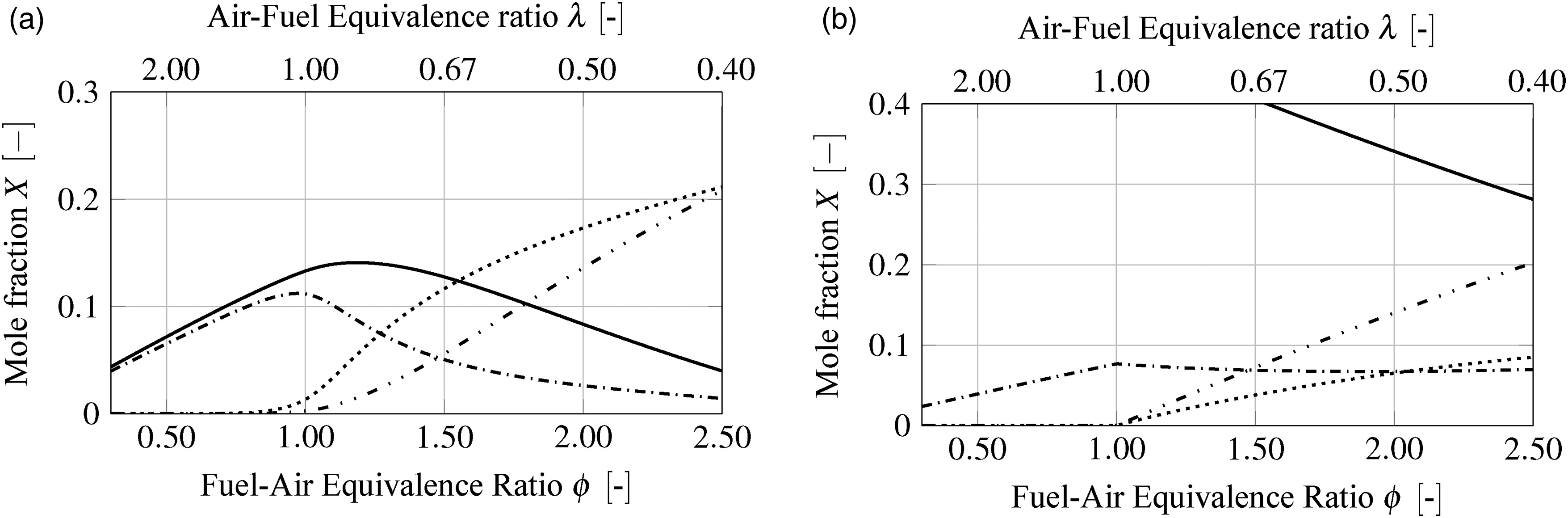
The results differ with the injection of steam. The decrease in temperature influences both exo- and endothermic reactions. After the stoichiometric point CO₂ remains constant while CO is still increasing as shown in Figure 6(b). Moreover, CO₂ and CO no longer balance each other. To address this effect at high WGR, H₂ is added in the progress variable definitions WETC1 and WETC2. WETC1 and WETC2 differ only in the weighting factor of hydrogen. The progress variable definition WETC3 allows a proper comparison to the description of Ma (2016), as it only differs in the weighting factor for H₂O.

The source term of the progress variable is illustrated by color in the C−Z space in Figure 7. In 7(a) the peak is at stoichiometric conditions. The propagation in the direction of scaled progress variable is small compared to others. The conspicuous behavior in the right upper region can be explained by the high weighting factor of H₂O leading to a relatively small difference of YC,min and YC,max at a constant Z. This results in a stretched C with ambiguous manifolds. The DryNGC definition seems fine for high WGR. Noticeable is that the H₂O content is only implicitly represented by the temperature that effects CO and CO₂ emissions. The Z distribution is wider but the gradients in C direction are higher than the WETCs. As expected, the smallest deviations are present between the WETC1 Figure 7(c) and WETC2 Figure 7(d). However, the WETC2 shows a stronger spread to smaller C. The increase of the H₂ content by 0.25 shows a slight effect on the gradients of the source term. The effects are negligible. The comparison of 7(e) and 7(a) shows that the weighting factor wH2O is dominant at ultra WET conditions.

Figure 7.

Parameter study: Normalized progress variable source term of premixed flamelets T_in = 600 K, p = 20 bar and WGR = 0.3. (a) MaC (Ma, 2016). (b) DryNGC (Fiorina et al., 2003, 2005a,b). (c) WETC1. (d) WETC2. (e) WETC3.

https://journal.gpps.global/f/fulltexts/188264/JGPPS-00214-2023-01.07_min.jpg

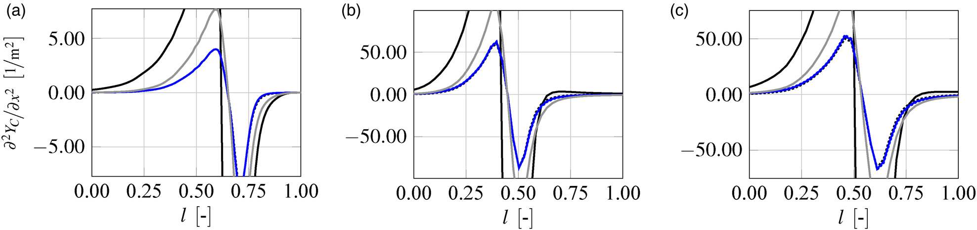
In contrast to the qualitative consideration in Figure 7 the second derivative of YC is examined for the conclusive determination in Figure 8. For this purpose, three premixed flames are simulated at Zlean Figure 8(a), Zst Figure 8(b) and Zlean Figure 8(c) for all variations of YC. The second derivative describes the curvature of the profile and thus the change of the gradient at a constant Z. It should be noticed that at low values of the second derivative a continuous gradient is present. From this, a more accurate prediction of the source term in a numerical simulation can be inferred. The results reflect the phenomena already identified. The curvature change at MaC is high at all conditions. The additional fraction of wCO2 increases especially in the rich region WETC3 in 8(c). The combination of the considerations leads to the progress variable WETC2, which is used in the following.

Figure 8.

Curvature of progress variable vs. normalized length, (MaC ), (DryNGC ), (WETC1 ), (WETC2 ) and (WETC3 ) at lean, stoichiometric and rich conditions T_in = 600 K, p = 20 bar and WGR = 0.3. (a) Z_lean. (b) Z_st. (c) Z_rich.

https://journal.gpps.global/f/fulltexts/188264/JGPPS-00214-2023-01.08_min.jpg

Progress variable source term distribution

Dry combustion

The normalized source term of the progress variable is illustrated in Figure 9 with a threshold to show only the area of interest. Under dry conditions differences are seen especially in the mixture fraction. Due to diffusion and the mixing between the oxidizer and fuel the non-premixed flamelets extend to higher Z values. Nerveless, the reaction area is smaller compared to the premixed. The deviation shown has no influence on the stoichiometric point. As a result, the position of the maximum value of the source term is identical for dry non-premixed and premixed flamelets.

Figure 9.

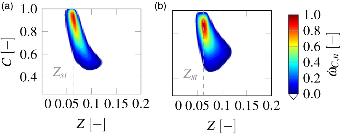
Normalized progress variable source term of premixed and non-premixed flamelets WETC2 at dry combustion condition T_in = 600 K, p = 20 bar and WGR = 0.0. (a) Premixed. (b) Non-Premixed.

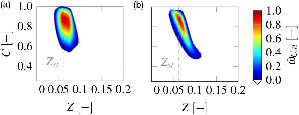
https://journal.gpps.global/f/fulltexts/188264/JGPPS-00214-2023-01.09_min.jpg

If the results shown in Figures 9(a) and 9(b) are compared with Hansinger et al. (2017) the differences are significant. The discrepancy may result from two aspects i.e., the higher pressure and inlet temperature at aero engine conditions in the present study. Qiao et al. (2021) have shown for a different fuel that increasing the pressure and temperature results in a further expansion of the maximum temperature depending on the strain rate. For high pressures, the maximum temperature is increasing while the strain rate is increasing. Therefore, the pressure increase has an effect mainly on the counterflow diffusion flame used in the non-premixed case. The increase in temperatures results in a constant maximum temperature at higher strain rates. It is assumed that this effect also occurs with the fuel kerosene. As a result the quenching strain rate increases with higher pressures and inlet temperatures. Thus, the formation of the flamelets in the non-premixed case is more influenced compared to the premixed case. The impact is seen in an expansion of the source term of the non-premixed flamelets to lower progress variable values in Figure 9(b). In addition, the applied fuel is different which has also an influence on different characteristics of the flamelets.

WET combustion

Under WET conditions, the generation of non-premixed flamelets in particular involves a certain amount of user effort compared to premixed flamelets. The Steam injection reduces the steady branch of the non-premixed flamelets, where the unsteady branch has a higher impact. Figure 10 shows the influence of steam injection with a WGR of 10% on the source term of the progress variable. The increase of the water content in the flamelets implies a decrease in temperature. The reduction of CO in both cases narrows the distribution in mixture fraction space. Furthermore, the steam is impacting the progress variable. The progress variable includes H₂ which is affected less than the other species at low WET conditions. The different behavior of the two models is due to the same effects under dry conditions. The quenching is reducing the flame temperature and the flame thickness of the non-premixed flame. Water content enhances this effect. The result is a lower temperature gradient at a constant mixture fraction compared to the premixed flamelets. This is expressed in the source term as a wider peak area.

Figure 10.

Normalized progress variable source term of premixed and non-premixed flamelets WETC2 at WET combustion condition T_in = 600 K, p = 20 bar and WGR = 0.1. (a) Premixed. (b) Non-Premixed.

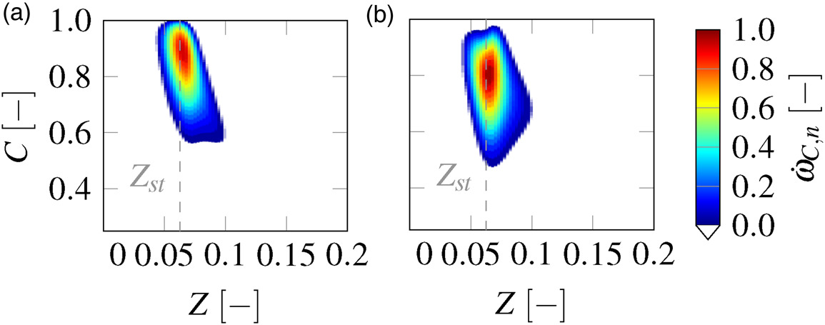
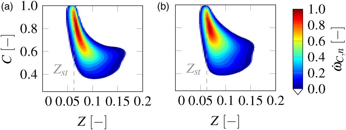
https://journal.gpps.global/f/fulltexts/188264/JGPPS-00214-2023-01.10_min.jpg

Figures 11(a) and 11(b) illustrate the representation of the different manifolds at a WGR of 0.2. The further increase of the steam content changes the impact of H₂. From dry to higher wet conditions the distribution for the premixed case expand to lower progress variable values.

Figure 11.

Normalized progress variable source term of premixed and non-premixed flamelets WETC2 at WET combustion condition T_in = 600 K, p = 20 bar and WGR = 0.2. (a) Premixed. (b) Non-Premixed.

https://journal.gpps.global/f/fulltexts/188264/JGPPS-00214-2023-01.11_min.jpg

The source terms for ultra WET conditions at WGR=0.3 are shown in Figure 12. With the high amount of steam and the adiabatic flame temperature reduction the intersection point of CO and CO₂ in the equivalence ratio space are shifted to higher values explained in Figure 6(b). This results in a stronger dominance of H₂ and an increase of the range to larger mixture fractions depending on the definition of the progress variable. Moreover, it can be seen in a qualitative comparison that the defined normalized progress variable favors the manifolds in both cases. The total area is larger and the gradients in source terms are greatly reduced. The trend of the differences between premixed and non-premixed are also seen with the further increase of steam. However, it seems that the discrepancies are greater with higher steam content, especially in the centre of the maximum source term. At this point, it would be useful to perform a further analysis of the influence of steam on the strain rate.

Figure 12.

Normalized progress variable source term of premixed and non-premixed flamelets WETC2 at ultra WET combustion condition T_in = 600 K, p = 20 bar and WGR = 0.3. (a) Premixed. (b) Non-Premixed.

https://journal.gpps.global/f/fulltexts/188264/JGPPS-00214-2023-01.12_min.jpg

Numerical verification case

Sandia flame D

In order to verify the progress variable approach and illustrate the three-dimensional effects of the premixed and non-premixed flamelets an academic jet flame “Sandia Flame” by Barlow and Frank (1998), Barlow et al. (2005) and Schneider et al. (2003) is used. They experimentally investigated the flame on various operating points and provided the data in the International Workshop on Measurement and Computation of Turbulent Flames (TNF) (TNF, 2023). In this work the configuration Sandia Flame D, a methane-air flame, is used for the validation of the numerical modelling. In addition, the verification process is carried out in three stages. First, the numerical model is validated using the original Sandia Flame D configuration. This is done by comparing the numerical results of the premixed and non-premixed flames with the experimental results. Subsequently, the aero engine relevant dry operating conditions are set. To characterize the behavior of the premixed and non-premixed flamelets, the results from the dry case are compared with the original Sandia Flame D case. Finally, steam is injected and the effect on the premixed and non-premixed manifolds is analyzed. This procedure ensures that a first statement about the behavior of premixed and non-premixed flamelets in aero engine applications with high steam is possible without an additional experiment.

Validation case and numerical setup

The Sandia Flame D is a piloted coaxial turbulent methane-air diffusion flame with three inlet streams. The main jet is characterized by a equivalence ratio of ϕ=3.17/Z=0.1559, the pilot jet by a burned mixture of ϕ=0.77/Z=0.0429 and the co-flow by ϕ=0/Z=0 contains only oxidizer. Therefore, the Sandia Flame D covers a wide range of equivalence ratios and flame regimes, which makes it suitable as a validation case for premixed and non-premixed flamelets. To resolve the dissipation of the vortices and the break-up of the jet, a LES simulation is used with the subgrid model Smagorinsky (1963). The domain is discretized with a structured hexahedral grid with 10.4 million cells. For the main jet flow and the shear layer between the pilot and main flow a maximum lateral cell size of 0.2mm and longitudinal of 1.1mm is chosen. Near the wall of the pipe, the grid is refined to resolve the turbulent boundary layer of the flow with a Re of 22400. In the annular duct of the pilot stream is the grid coarser respectively to the lower Re of 315. The selection of the mesh is the result of an independence study on the basis of Celik et al. (2008) and Pope (2000). The employed discretization schemes are second order in time and space. For the main inlet, a fully developed turbulent pipe flow is time-mapped to the Sandia Flame D simulation. Since the flow of the annular duct is laminar, a constant field is set at the pilot inlet. The velocity conditions are stay the same for all three cases. For the kerosene case the inlet temperature and pressure are set to aero engine conditions. The cases are listed in Table 4. For the original Sandia Flame D case with CH₄, the GRI3.0 mechanism with 53 species and 325 reaction equations is used for the generation of premixed and non-premixed flamelets (Smith et al., 2023). From the analyses in the previous chapter, the original Dag_LP mechanism was found to be the best solution of the chemical mechanisms investigated, in addition to the POLIMI as a reference. The Dag_LP is used due to the reduction in pre-processing computational time. Under the conditions shown in Table 4, kerosene is assumed to be gaseous.

Table 4.

Simulation cases.

Case Name	Fuel	Tmain(K)	ϕmain/Z(−)	ϕpilot/Z(−)	p(bar)	WGR(−)
Org. Sandia Flame D^a	CH₄	294	3.17/0.1559	0.77/0.0429	1	0.00
Dry aero engine conditions (DryAEC)	C₁₀H₂₂	600	3.17/0.1748	0.77/0.0490	20	0.00
Ultra WET aero engine conditions (WetAEC)	C₁₀H₂₂	600	3.17/0.1292	0.90/0.0404	20	0.30

[i] ^aBarlow and Frank (1998), Schneider et al. (2003) and Barlow et al. (2005).

To simulate the reacting flow, the FGM combustion model mentioned above is implemented in OpenFOAM. The two independent variables C~ and Z~ are supplemented by an assumed β-PDF approach with the corresponding variances C′′2~ and Z′′2~. Consequently, a four-dimensional look-up table is accessed during the simulation. In this model, only the mean values of the unscaled progress variable and the mixture fraction are transported. The variances are calculated using a dynamic algebraic model (Ma, 2016).

Results

Methane-air sandia flame D

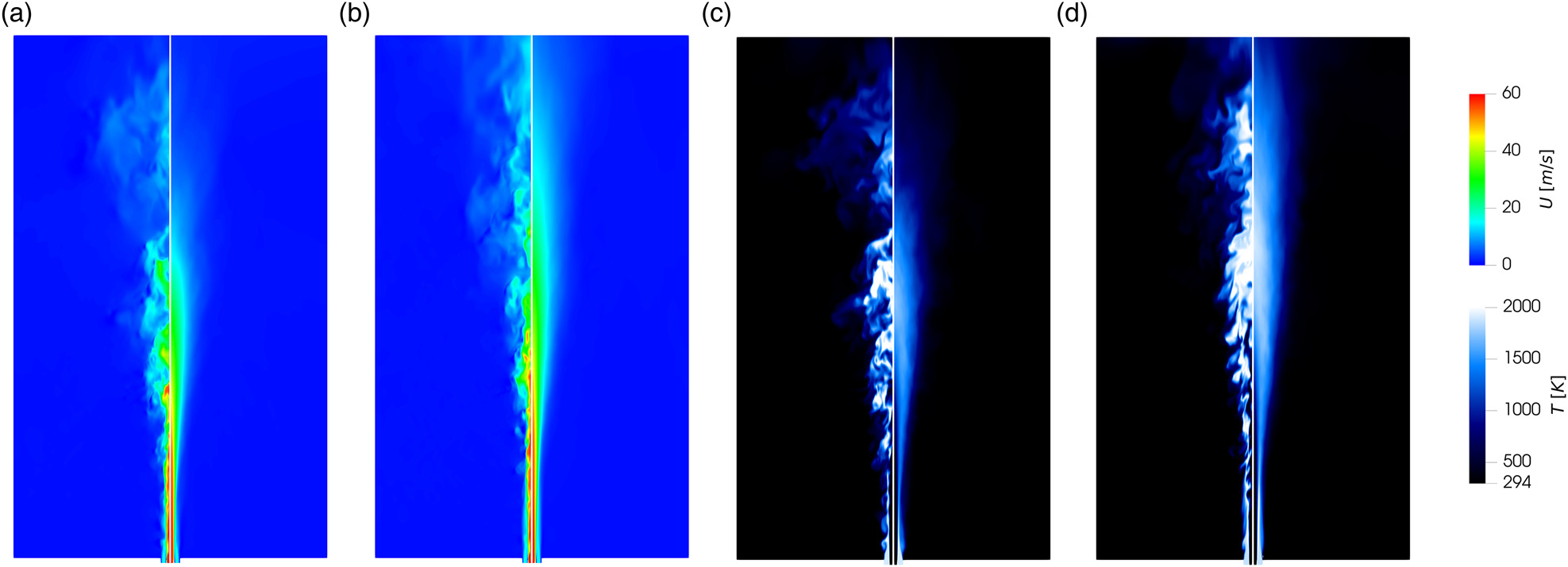
With respect to the flame structure, the instantaneous distribution of velocity and temperature, as well as the corresponding mean values, are considered quantitatively. Similar structures can be seen in the velocity distributions of the premixed and non-premixed results in Figures 13(a) and 13(b). The instantaneous snapshot shows the vorticities of the jet. In the mean field it is evident that the break-up widens the jet and increases the temperature and velocity fluctuations. This behavior can be seen in both cases. Nerveless, the penetration depth is lower with premixed flamelets. It follows that the break-up of the jet is evident at low axial positions and the kinetic energy of the vortices dissipates earlier.

Figure 13.

Instantaneous (left) and mean (right) axial velocity and temperature distribution of Sandia Flame D. (a) Premixed axial velocity distribution. (b) Non-premixed axial velocity distribution. (c) Premixed temperature distribution. (d) Non-premixed temperature distribution.

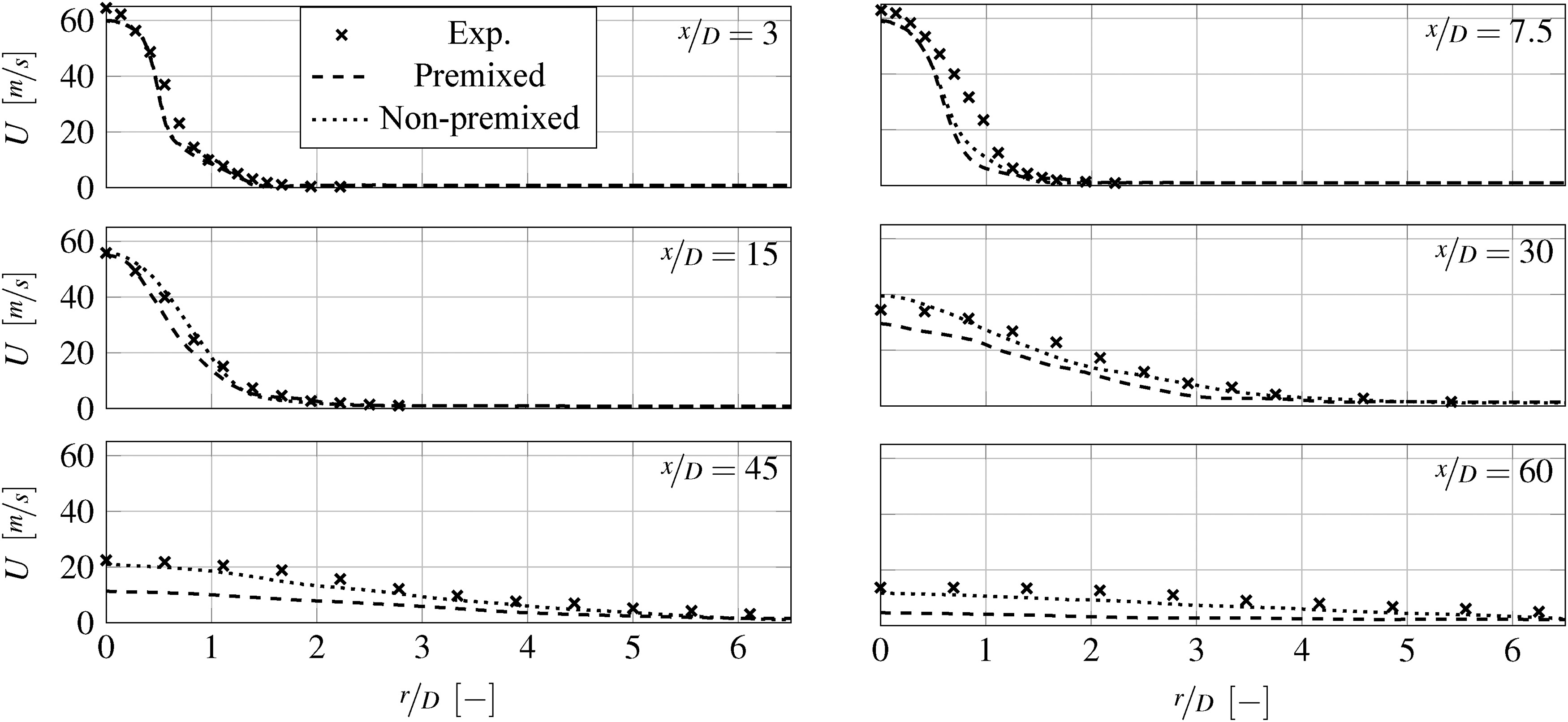
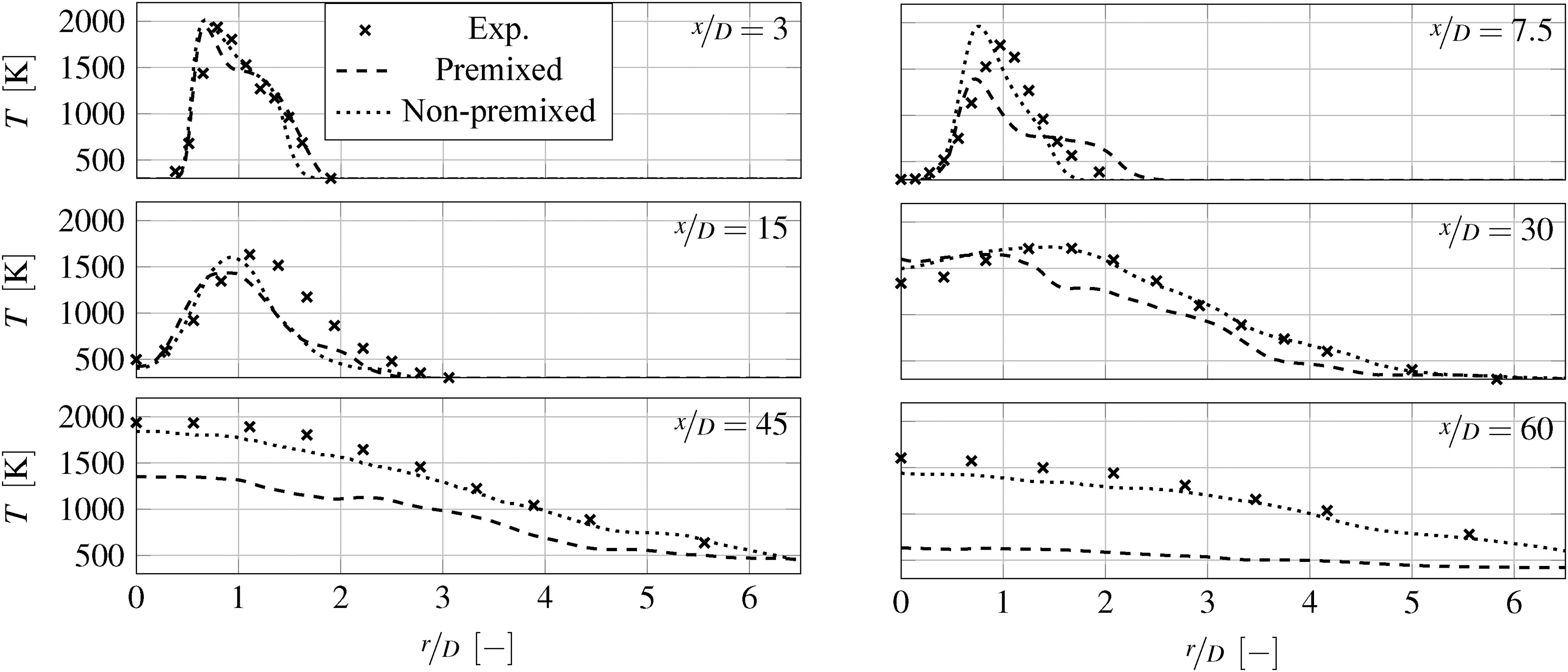
https://journal.gpps.global/f/fulltexts/188264/JGPPS-00214-2023-01.13_min.jpg

For the validation of the numerical model, certain axial positions along the main flow direction are used. In order to consider the full range, the radial temperature and axial velocity distributions are shown over the axial positions x/D = 3, 7.5, 15 and 30. Figure 14 shows a good agreement between the non-premixed and the experimental results with an error of less than 5% when x/d = 7.5 is not taken into account. Contrary to the seemingly different contour plots, the radial profile shows a better agreement between the cases. This is due to the chosen axial positions. The premixed model is not able to reproduce the jet break-up and associated temperature distribution based on Z and C as well as the non-premixed model, but the overall agreement is still good. The profiles at x/D = 30 are particularly representative of this characteristic. The trend of the temperature profiles is reflected by both premixed and non-premixed. The radial shift at lower x/D of the simulation results is noticeable. The almost identical agreement of the non-premixed profile at x/D = 30 stands out in Figure 15. Overall, the comparison with the results shows a validation of the implementation of the FGM model. In particular, the results with the non-premixed flamelets are in good agreement with the analysis of Mahmoud (2020). Therefore, the results obtained by Hansinger et al. (2017) could not be confirmed using the Sandia Flame D. They showed a better agreement between the experimental and premixed flamelet results. The RMS values are not explicitly presented in this paper, but they showed good overall agreement.

Figure 14.

Radial velocity profiles at various axial positions x/D of Sandia Flame D.

https://journal.gpps.global/f/fulltexts/188264/JGPPS-00214-2023-01.14_min.jpg

Figure 15.

Radial temperature profiles at various axial positions x/D of Sandia Flame D.

https://journal.gpps.global/f/fulltexts/188264/JGPPS-00214-2023-01.15_min.jpg

Kerosene-air sandia flame

The focus in this paper is on the application of premixed and non-premixed flamelets in aero engine conditions, especially with high steam content. For this purpose, the generated flamelets are first examined under dry conditions. Three things in particular are discussed here: The influence of the high temperature, the high pressure and the characteristics of kerosene.

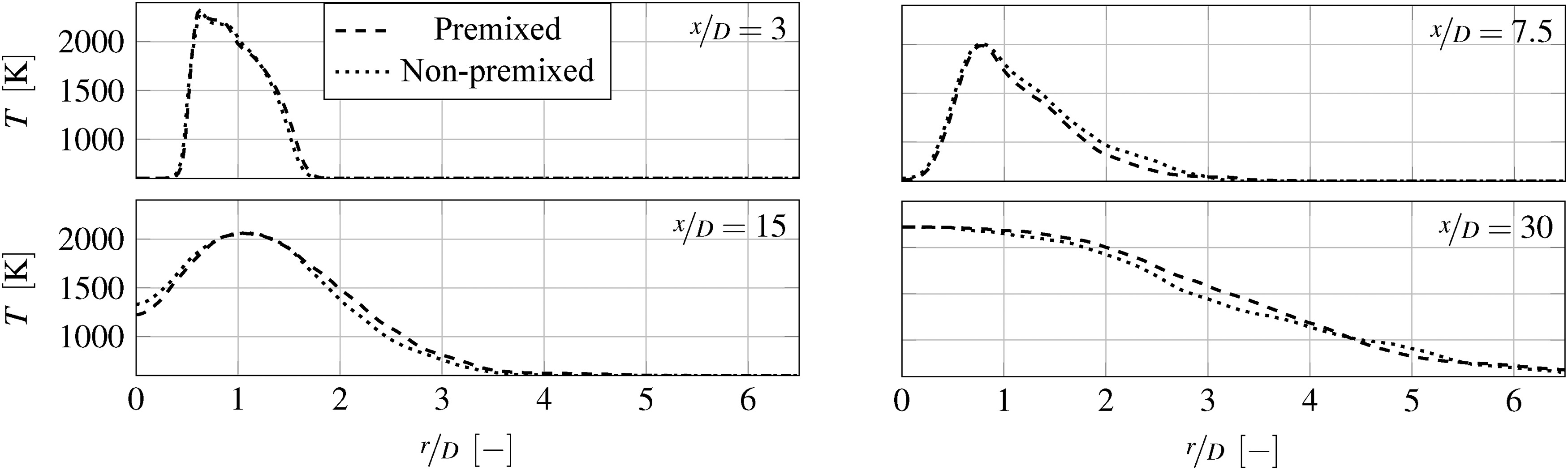
The DryAEC conditions in Figure 16 show a wider radial velocity and temperature expansion and therefore, a break-up of the main jet at a lower axial position. The process of the jet break-up is influenced by various factors, including the fuel and oxidizer properties, turbulence intensity and chemistry. Close to the nozzle of the burner, Kelvin-Helmholtz instabilities occur between the co-flow and pilot stream in both simulations. Due to the higher ratio of the pilot and co-flow temperature the intensity of this phenomenon is greater than in the methane case discussed above. Apart from that, the axial expansion of the temperature is lower, which indicates the influence of high pressure, fuel characteristics and inlet temperature.

Figure 16.

Instantaneous (left) and mean (right) axial velocity and temperature distribution of DryAEC Sandia Flame. (a) Premixed axial velocity distribution. (b) Non-premixed axial velocity distribution. (c) Premixed temperature distribution. (d) Non-premixed temperature distribution.

https://journal.gpps.global/f/fulltexts/188264/JGPPS-00214-2023-01.16_min.jpg

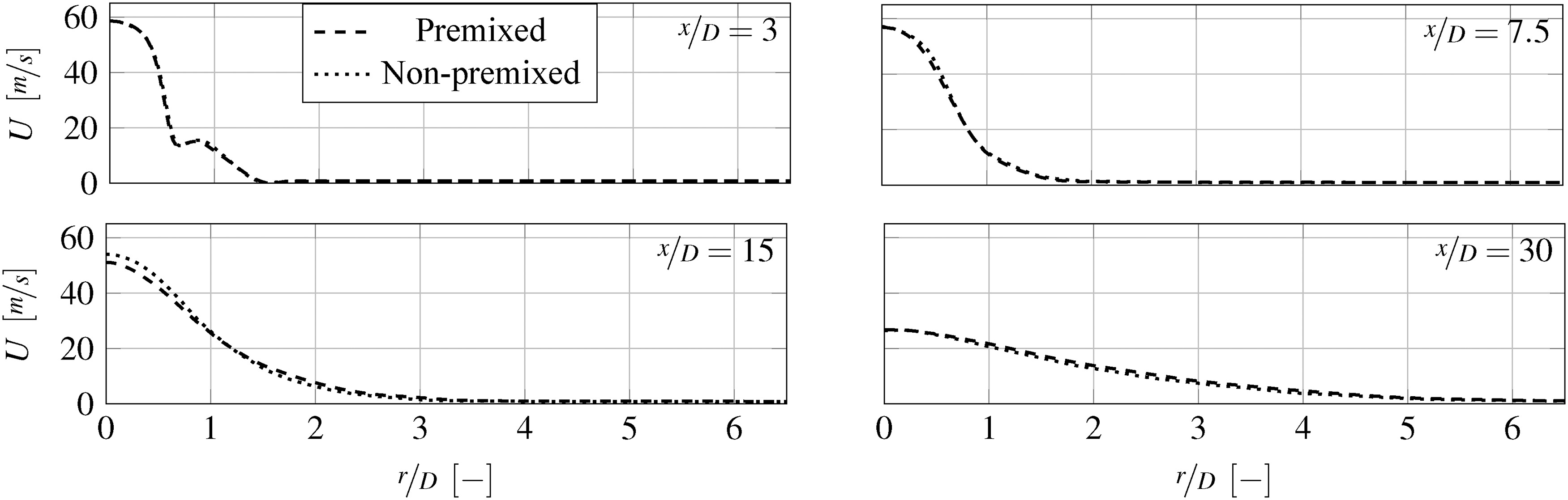
With the exception of x/D = 3, there are no major differences in the trend of the velocity profiles shown in Figure 17. This can be explained by the fact that the inlet velocities are the same as those of the Sandia Flame D. At x/D=3 the shear layer between the main and pilot flow is clearly visible as a kink in the profiles. The temperature profiles of premixed and non-premixed case feature almost identical characteristics. The premixed simulation tends to have a slightly lower temperature in the shear layer and does not match with the non-premixed results in Figure 18.

Figure 17.

Radial velocity profiles at various axial positions x/D of DryACE Sandia Flame.

https://journal.gpps.global/f/fulltexts/188264/JGPPS-00214-2023-01.17_min.jpg

Figure 18.

Radial temperature profiles at various axial positions x/D of DryACE Sandia Flame.

https://journal.gpps.global/f/fulltexts/188264/JGPPS-00214-2023-01.18_min.jpg

Kerosene-air-steam sandia flame

The additional steam significantly decreases the flame length. When steam is injected, the equivalence ratio at the main inlet is kept constant and the mass of the fuel-air mixture is reduced by the amount of steam. This consideration inevitably results in a reduction of the thermal power. As a result, the impulse in the domain is reduced. The opposite approach, where the thermal power is independent of the amount of steam, is explored by Hiestermann et al. (2022).

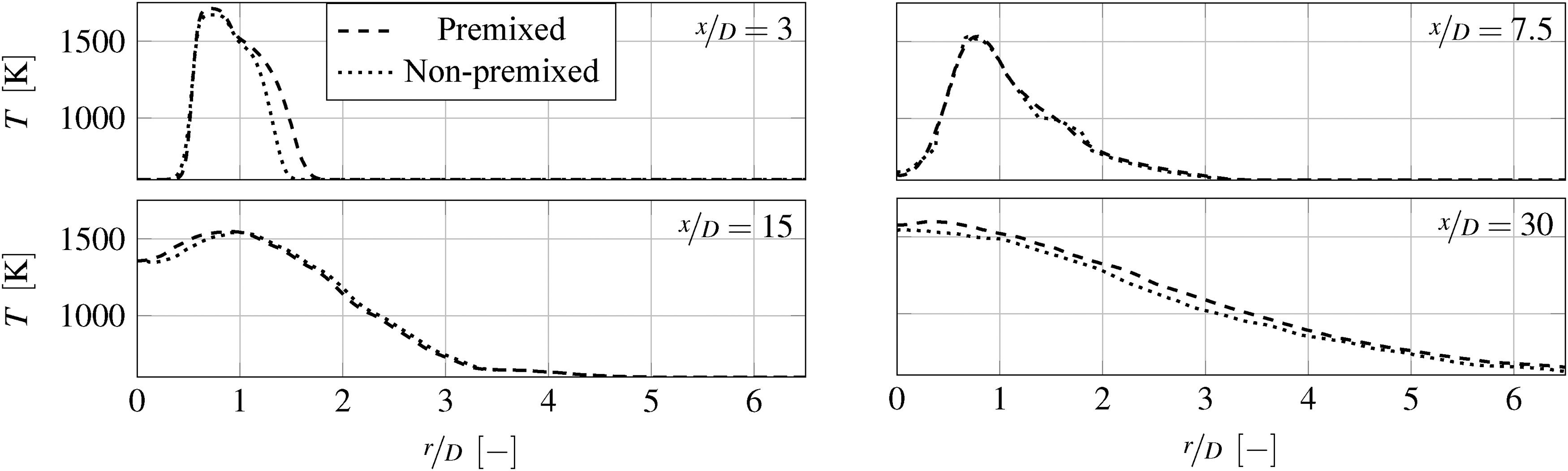
For the WET conditions the flame had to be stabilized by a higher equivalence ratio at the pilot inlet. The reason for that is the strong reduction of the adiabatic flame temperature due to the high amount of steam on the oxidizer side. This is shown in Figure 2. Compared to the previous simulation, it is noticeable that the premixed and non-premixed results are significantly closer to each other in Figure 19. The addition of steam has the effect that the thermal diffusivity is increased by a higher specific heat capacity of the mixture. The difference in the assumption of a freely propagating flame and a counter flow diffusion flame is thus reduced. This is supported by the similar penetration depth of the jet into the domain as well as the absolute axial length of the temperature distribution. Likewise of the counterplots are the radial velocity profilesin Figure 20. As in the previous observation, the trend is similar to that of the Sandia Flame D. However, it should be noted that the peak of the velocity at x/D = 30 is lower compared to the dry case. This occurs even though the inlet velocities are identical. The temperature profiles show a slight offset between the two flamelet variants illustrated in Figure 21.

Figure 19.

Instantaneous (left) and mean (right) axial velocity and temperature distribution of WetAEC Sandia Flame. (a) Premixed axial velocity distribution. (b) Non-premixed axial velocity distribution. (c) Premixed temperature distribution. (d) Non-premixed temperature distribution.

https://journal.gpps.global/f/fulltexts/188264/JGPPS-00214-2023-01.19_min.jpg

Figure 20.

Radial velocity profiles at various axial positions x/D of WetAEC Sandia Flame.

https://journal.gpps.global/f/fulltexts/188264/JGPPS-00214-2023-01.20_min.jpg

Figure 21.

Radial temperature profiles at various axial positions x/D of WetAEC Sandia Flame.

https://journal.gpps.global/f/fulltexts/188264/JGPPS-00214-2023-01.21_min.jpg

Conclusion

This study focuses on the influence of the selected one-dimensional model flame setup for flamelet-generated manifold (FGM) combustion large eddy simulations (LES) at ultra WET aero engine conditions. Various mechanisms for kerosene combustion investigated at aero engine conditions represent the influence of steam injection on the reaction kinetics with different degrees of accuracy. Even for detailed mechanisms, like Dagaut (Dagaut, 2002; Dagaut and Cathonnet, 2006) and POLIMI (Ranzi et al., 1995, 2005), the predicted laminar flame speeds and particularly the obtained inner flame structures differ considerably. Hence, special attention must be paid to the selection of a reaction mechanism for ultra WET aero engine conditions.

The choice of the progress variable definition, especially the adjustment of the weighting coefficients for the species mass fractions, is crucial for a good representation of the manifolds. This study reveals that a single set of weighting factors is not sufficient for all considered dry to ultra WET aero engine operating conditions. We showed that particularly for ultra WET conditions a specific combination of H₂, CO and CO₂ results in a well-defined progress variable.

The comparison of the premixed freely propagating flame and the non-premixed counter flow diffusion flame shows a effect of the flamelet models. One of the essential conclusion is that steam is affecting the distribution and magnitude of the source term. As the amount of steam increases, the difference between premixed and non-premixed flamelets decreases.

Based on FGM-LES of a customized Sandia Flame D setup we demonstrate, that the influence of the choice of one-dimensional model flame on the CFD results varies, depending on the fuel and operating conditions. Using non-premixed flamelets is superior for the original Sandia Flame D case with methane. For an adapted kerosene Sandia Flame at aero engine conditions, however, both flamelet models yield almost identical result, especially at ultra WET conditions. The non-premixed flamelet approach is thus more reliable, but at the price of higher numerical and user effort compared to the premixed flamelet approach. While our results suggest, that at certain operating conditions premixed flamelets provide comparably good accuracy, the generalizability of this observation is still open to further research.

As a further study, the effect of steam on the strain rate sensitivity of premixed one-dimensional flames should be investigated. For this purpose, the model of the premixed counterflow flame can be applied to analyze strain rate. For the general application of premixed flamelets for dry and ultra WET aero engine condition, more configuration and operating points should be investigated. Furthermore, experiments should be carried out to validate the numerical model approaches for wet combustion.

Nomenclature

Roman letters

Speed of sound (m s¹)

Progress variable weighting factor (−)

Specific heat capacity (m s⁻²)

Scaled progress variable (−)

Diffusion coefficient (m² s⁻¹)

Diffusion mass fluxes (kmol m⁻² s⁻¹)

Number of atoms (−)

Pressure (bar)

Coordinate r axes (m)

Time (s)

Temperature (K)

Tad

Adiabatic flame temperature (K)

Molar enthalpy (J mol⁻¹)

Velocity component x (m s¹)

Axial velocity component (m s¹)

Velocity component y (m s¹)

Progress variable weighting factor (−)

Atomic mass (kg kmol⁻¹)

Coordinate x axes (m)

Molar fraction (−)

Coordinate y axes (m)

Mass fraction (−)

Progress variable (kmol kg⁻¹)

Coordinate z axes (m)

Mixture fraction (−)

Greek letters

Mass density (kg m⁻³)

Cylindrical/Cartesian factor (−)

Bilger coefficient (−)

Non-dimensional strain rate (−)

Thermal conductivity (W m⁻¹ K⁻¹)

Air-Fuel equivalence ratio (−)

Dynamic viscosity (kg m s⁻¹)

Kinematic viscosity (m² s⁻¹)

Unsteady factor (−)

ω˙k

Molar production rate of species k (kg m⁻³ s⁻¹))

ω˙C

Progress variable source term (kg m⁻³ s⁻¹)

Fuel-Air equivalence ratio or equivalence ratio (−)

Substitution groups

Potential flow substitution, uc/u∞

Superscripts and subscripts

Species of k

min

Minimal

max

Maximal

∞

Free stream

∼

mean

′′2~

variance

Appendix A. Governing Equations for Flamelets

The flamelets equations are based on the three-dimensional governing equations. With the assumption of axisymmetric stagnation flow the formulation can be reduced to one-dimensional equations, which describes the flamelets (Kee et al., 2017). In general the flamelet structures are a function of time represented by the value θ=1 in the continuity Equation (7), momentum Equation (8), species Equation (9) and energy Equation (10). Based on the flame model the description with cylindrical or cartesian coordinate is used described with α.

(7)

θ∂ρ∂t+1rα∂∂r(rαρν)+pU=0

(8)

θρ∂U∂t+ρU2+ρν∂U∂r=ρ∞dcdt+ρ∞c2+1rα∂∂r[rαμ∂U∂r]

(9)

θρ∂Yk∂t+VYk∂r=1rα∂∂r[rαjk]+ω˙kWk

(10)

θρ∂T∂t+ρv∂T∂r+1cp(∑k=1Kh^kω˙k+∑k=1Kjkcp,k∂T∂r)=1cp1rα∂∂r[rακ∂T∂r]

The energy Equation (10) and species Equation (9) includes the diffusive fluxes. In Equation (11) the species diffusive mass fluxes jk are described with mean molecular weight, mixture-averaged diffusion coefficient Dk,i and the mole fraction of species kXk. If the flame model is changed, the basic equations remain.

(11)

jk=ρWkW¯2∑i⁡WiDk,i∂Xi∂z

COMPETING INTERESTS

Marian Hiestermann declares that he has no conflict of interest. Matthias Haeringer declares that he has no conflict of interest. Marcel Dèsor declares that he has no conflict of interest. Wolfgang Polifke declares that he has no conflict of interest.

REFERENCES (47)

Bagheri G., Ranzi E., Pelucchi M., Parente A., Frassoldati A., and Faravelli T. (2020). Comprehensive kinetic study of combustion technologies for low environmental impact: MILD and OXY-fuel combustion of methane. Combustion and Flame. 212: 142–155. 10.1016/j.combustflame.2019.10.014.

CrossRef

Google Scholar

Barlow R. S. and Frank J. (1998). Effects of turbulence on species mass fractions in methane/air jet flames. Symposium (International) on Combustion. 27: 1087–1095. 10.1016/S0082-0784(98)80510-9.

CrossRef

Google Scholar

Barlow R. S., Frank J., Karpetis A. N., and Chen J.-Y. (2005). Piloted methane/air jet flames: Transport effects and aspects of scalar structure. Combustion and Flame. 143: 433–449. 10.1016/j.combustflame.2005.08.017.

CrossRef

Google Scholar

Bilger R. (1989). The structure of turbulent nonpremixed flames. Symposium (International) on Combustion. 22 (1): 475–488. 10.1016/S0082-0784(89)80054-2.

CrossRef

Google Scholar

Bilger R. W. (1980a). Turbulent flows with nonpremixed reactants. Berlin, Heidelberg: Springer Berlin Heidelberg.

Google Scholar

Bilger R. W. (1980b). Turbulent Reacting Flows. In: Topics in Applied Physics, 1st ed. Berlin, Heidelberg: Springer Berlin Heidelberg, Vol. 44, pp. 65–113. Chapter Turbulent flows with nonpremixed reactants.

Google Scholar

Celik I. B., Ghia U., Roache P. J., Freitas C. J., Coleman H., and Raad P. E. (2008). Procedure for Estimation and Reporting of Uncertainty Due to Discretization in CFD Applications. Journal of Fluids Engineering. 130: 078001-1–4.

Google Scholar

Cerfacs (2023). Luches Mechanism. https://chemistry.cerfacs.fr/en/chemical-database/mechanisms-list/luches-mechanism/

WWW

Google Scholar

Dagaut P. (2002). On the kinetics of hydrocarbons oxidation from natural gas to kerosene and diesel fuel. Physical Chemistry Chemical Physics 4: 2079–2094. 10.1039/b110787a.

CrossRef

Google Scholar

10.

Dagaut P. and Cathonnet M. (2006). The ignition, oxidation, and combustion of kerosene: A review of experimental and kinetic modeling. Progress in Energy and Combustion Science. 32 (1): 48–92. 10.1016/j.pecs.2005.10.003.

CrossRef

Google Scholar

11.

Fiorina B., Baron R., Gicquel O., Thevenin D., Carpentier S., and Darabiha N. (2003). Modelling non-adiabatic partially premixed flames using flame-prolongation of ILDM. Combustion Theory and Modelling. 7 (3): 449–470. 10.1088/1364-7830/7/3/301.

CrossRef

Google Scholar

12.

Fiorina B., Gicquel O., Vervisch L., Carpentier S., and Darabiha N. (2005a). Approximating the chemical structure of partially premixed and diffusion counterflow flames using FPI flamelet tabulation. Combustion and Flame. 140 (3): 147–160. 10.1016/j.combustflame.2004.11.002.

CrossRef

Google Scholar

13.

Fiorina B., Gicquel O., Vervisch L., Carpentier S., and Darabiha N. (2005b). Premixed turbulent combustion modeling using tabulated detailed chemistry and PDF. Proceedings of the Combustion Institute. 30 (Part 1): 867–874. 10.1016/j.proci.2004.08.062.

CrossRef

Google Scholar

14.

Goodwin D. G., Moffat H. K., Schoegl I. L., Speth R., and Weber B. W. (2022). Cantera: An Object-oriented Software Toolkit for Chemical Kinetics, Thermodynamics, and Transport Processes. Version 2.6.0. https://www.cantera.org.

WWW

Google Scholar

15.

Göke S. (2012). Ultra Wet Combustion: An Experimental and Numerical Study. PhD thesis, Berlin, Germany: Technical University Berlin.

Google Scholar

16.

Hansinger M., Müller M., and Pfitzner M. (2017). Comparison of premixed and non-premixed manifold representations in the LES of a piloted jet flame with inhomogeneous inlets. In Proceedings of the European Combustion Meeting 2017.

Google Scholar

17.

Hassa C. (2013). Partially Premixed and Premixed Aero Engine Combustors. Cambridge Aerospace Series, Cambridge: Cambridge University Press, pp. 237–289.

Google Scholar

18.

Hiestermann M., Konle M., and de Guillebon L. (2022). Numerical investigation of the effect of high steam loads on the combustion of an academic premixed siwrl stabilized combustor. In Proceedings of Global Power and Propulsion Society, pp. GPPS-TC-2022-0094.

Google Scholar

19.

Ihme M. and Pitsch H. (2008). Prediction of extinction and reignition in nonpremixed turbulent flames using a flamelet/progress variable model: 1. A priori study and presumed PDF closure. Combustion and Flame. 155 (1): 70–89. 10.1016/j.combustflame.2008.04.001.

CrossRef

Google Scholar

20.

Ihme M., Shunn L., and Zhang J. (2012). Regularization of reaction progress variable for application to flamelet-based combustion models. Journal of Computational Physics. 231 (23): 7715–7721. 10.1016/j.jcp.2012.06.029.

CrossRef

Google Scholar

21.

Kaiser S., Schmitz O., Ziegler P., and Klingels H. (2022). The water-enhanced turbofan as enabler for climate-neutral aviation. Applied Sciences. 12 (23): 12431. 10.3390/app122312431.

CrossRef

Google Scholar

22.

Kee R. J., Coltrin M. E., Glarborg P., and Zhu H. (2017). Chemically Reacting Flow: Theory, Modeling, and Simulation, 2nd ed., Hoboken, NJ: Wiley.

Google Scholar

23.

Luche J. (2003). Obtention de modèles cinétiques réduits de combustion Application à un mécanisme du kérosène. Thèse de doctorat, université d’Orléan, PhD thesis, Universite D’orleans. https://chemistry.cerfacs.fr/wp-content/uploads/sites/76/2018/08/These_LUCHE.pdf.

WWW

Google Scholar

24.

Ma L. (2016). Computational Modeling of Turbulent Spray Combustion. PhD thesis, Delft, NL: Delf University of Technology.

Google Scholar

25.

Mahmoud R. (2020). Development and Application of an Eulerian Density Function Methodology Coupled to Flamelet Progress Variable Approach for the Simulation of Oxyfuel Combustion. PhD thesis, TU Darmstadt. https://tuprints.ulb.tu-darmstadt.de/17635/1/PhD-Thesis_Rihab_Mahmoud_TUD_2021.pdf.

WWW

Google Scholar

26.

Panchal A., Ranjan R., and Menon S. (2019). A comparison of finite rate kinetics and flamelet-generated manifold using a multiscale modeling framework for turbulent premixed combustion. Combustion Science and Technology 191 (5–6): 921–955.

Google Scholar

27.

Peters N. (1984). Laminar diffusion flamelet models in non-premixed turbulent combustion. Progress in Energy and Combustion Science. 10 (3): 319–339. 10.1016/0360-1285(84)90114-X.

CrossRef

Google Scholar

28.

Peters N. (1988). Laminar flamelet concepts in turbulent combustion. Symposium (International) on Combustion. 21 (1): 1231–1250. Twenty-First Symposuim (International on Combustion). 10.1016/S0082-0784(88)80355-2.

CrossRef

Google Scholar

29.

Peters N. and Kee R. (1987). The computation of stretched laminar methane-air diffusion flames using a reduced four-step mechanism. Combustion and Flame. 68 (1): 17–29. 10.1016/0010-2180(87)90062-9.

CrossRef

Google Scholar

30.

Pitsch H. and Ihme M. (2005). An unsteady flamelet progress variable method for LES of nonpremixed turbulent combustion. In 43rd AIAA Aerospace Sciences Meeting and Exhibit, 43, pp. AIAA 2005-557. https://arc.aiaa.org/doi/abs/10.2514/6.2005-557.

WWW

Google Scholar

31.

Pope S. B. (2000). Turbulent Flows. Cambridge: Cambridge University Press.

Google Scholar

32.

Qiao Z., Lv Y., and Hickey J.-P. (2021). Single-phase instability of intermediate flamelet states in high-pressure combustion. Fuel. 288: 119736. 10.1016/j.fuel.2020.119736.

CrossRef

Google Scholar

33.

Ramaekers W., Albrecht B., van Oijen J., de Goey L., and Eggels R. (2005). The application of flamelet generated manifolds in partailly-premixed flames. In Proceedings of the Fluent Benelux User Group Meeting, 6–7 October 2005, Wavre, Belgium. https://research.tue.nl/nl/publications/predicting-no-formation-with-flamelet-generated-manifolds.

WWW

Google Scholar

34.

Ranzi E., Gaffuri P., Faravelli T., and Dagaut P. (1995). A wide-range modeling study of n-heptane oxidation. Combustion and Flame. 103 (1): 91–106. 10.1016/0010-2180(95)00091-J.

CrossRef

Google Scholar

35.

Ranzi E., Frassoldati A., Granata S., and Faravelli T. (2005). Wide-range kinetic modeling study of the pyrolysis, partial oxidation, and combustion of heavy n-alkanes. Industrial & Engineering Chemistry Research. 44 (14): 5170–5183. 10.1021/ie049318g.

CrossRef

Google Scholar

36.

Ranzi E., Frassoldati A., Grana R., Cuoci A., Faravelli T., et al. (2012). Hierarchical and comparative kinetic modeling of laminar flame speeds of hydrocarbon and oxygenated fuels. Progress in Energy and Combustion Science. 38 (4): 468–501. 10.1016/j.pecs.2012.03.004.

CrossRef

Google Scholar

37.

Ranzi E., Frassoldatti A., Stagni A., Peluchi M., Cuoci A., and Faravelli T. (2014). Reduced kinetic schemes of complex reaction systems: Fossil and biomass-derived transportation fuels. International Journal of Chemical Kinetics. 46 (9): 512–542. 10.1002/kin.20867.

CrossRef

Google Scholar

38.

Ranzi E., Cavallotti C., Cuoci A., Frassoldati A., Pelucchi M., and Faravelli T. (2015). New reaction classes in the kinetic modeling of low temperature oxidation of n-alkanes. Combustion and Flame. 162 (5): 1679–1691. 10.1016/j.combustflame.2014.11.030.

CrossRef

Google Scholar

39.

Schimek S., Göke S., and Paschereit C. O. (2013). Emission formation of liquid fuel combustion under humidied conditions, AIAA 2013-0693, 51, pp. AIAA 2013-0693.

Google Scholar

40.

Schmitz O., Kaiser S., Klingels H., Kufner P., Obermueller M., et al. (2020). Aero engine concepts beyond 2030: Part3 – experimental demonstration of technological feasibilty. In ASME Turbo Expo 2020.

Google Scholar

41.

Schneider C., Dreizler A., Janicka J., and Hassel E. P. (2003). Flow field measurements of stable and locally extinguishing hydrocarbon-fuelled jet flames. Combustion and Flame. 135: 185–190. 10.1016/S0010-2180(03)00150-0.

CrossRef

Google Scholar

42.

Smagorinsky J. (1963). General circulation experiments with the primitive equations. Monthly Weather Review. 91: 99–164. 10.1175/1520-0493(1963)091<0099:GCEWTP>2.3.CO;2.

CrossRef

Google Scholar

43.

Smith G. P., Golden D. M., Frenklach M., Moriarty N. W., Eiteneer B., et al. (2023). GRI-Mech 3.0. http://www.me.berkeley.edu/gri_mech/.

WWW

Google Scholar

44.

Speth L. R. (2022). Ember unsteady reacting flow solver. https://speth.github.io/ember-doc/sphinx/html/index.html.

WWW

Google Scholar

45.

TNF (2023). International Workshop on Measurement and Computation of Turbulent Flames. https://tnfworkshop.org/.

WWW

Google Scholar

46.

Wu Y., Modica V., Yu X., and Grisch F. (2018). Experimental investigation of laminar flame speed measurement for kerosene fuels: jet A-1, surrogate fuel, and its pure components. Energy & Fuels. 32 (2): 2332–2343. 10.1021/acs.energyfuels.7b02731.

CrossRef

Google Scholar

47.

Yang S., Wang X., Sun W., and Huo H. (2017). Comparison of flamelet/progress-variable and finite rate chemistry LES models in a preconditioning scheme. In AIAA SciTech Forum.

Journal Issues

Indexes

Table of contents

Introduction Chemical mechanism Progress variable study Progress variable source term distribution Numerical verification case Results Conclusion Nomenclature Appendix A. Governing Equations for Flamelets COMPETING INTERESTS REFERENCES

Introduction

Chemical mechanism

Table 1.

Chemical mechanisms for long-chain hydrocarbon fuel.

Operating points

Table 2.

Operating conditions from dry to ultra WET.

(1)

Laminar flame speed

Figure 1.

Laminar flame speed vs. equivalence ratio WGR symbols: (+ WGR = 0.00), ( WGR = 0.10), ( WGR = 0.20), ( WGR = 0.30), chemical mechanism colors: ( Luche), ( DagHP), ( DagLP), ( POLIMI), Tad = 1,800 K, Tin = 600 K, p = 20 bar.

Figure 2.

Adiabatic flame temperature vs. equivalence ratio for (One-Step ), (Luche, DagLP and DagHP ) and (Polimi +) with WGR 0.0, 0.1, 0.2, 0.3 Tin = 600 K, p = 20 bar.

Concentration of carbon monoxide and dioxide

Figure 3.

Mole fraction vs. normalized length of CO () and CO2 (), chemical mechanism colors: ( Luche), ( DagHP), ( DagLP), ( POLIMI), Tad = 1,800 K, Tin = 600 K, p = 20 bar. (a) Dry combustion WGR = 0.00 at ϕ = 2.09. (b) Ultra WET combustion WGR = 0.30 at ϕ = 1.03.

Flame configuration

Figure 4.

Flame configurations. (a) Freely propagating flame. (b) Counterflow diffusion flame.

Flamelet table variables

(2)

(3)

(4)

(5)

(6)

Premixed: freely propagating flame

Figure 5.

Temperature vs. mixture fraction of premixed freely propagating flame and counterflow diffusion flame with normalized progress variable isolines. (a) Freely propagating flames. (b) Counterflow diffusion flames for steady and unsteady branches.

Non-premixed: counterflow diffusion flame

Progress variable study

Progress variable requirements

Progress variable definition

Table 3.

Progress variable definition.

Figure 6.

Molar fraction vs. equivalence ratio for (H2O ), (H2 ), (CO ) and (CO2 ) at Dry WGR 0.0 and ultra WET conditions 0.3 Tin = 600 K, p = 20 bar. (a) Dry combustion WGR = 0.00. (b) Ultra WET combustion WGR = 0.30.

Figure 7.

Parameter study: Normalized progress variable source term of premixed flamelets Tin = 600 K, p = 20 bar and WGR = 0.3. (a) MaC (Ma, 2016). (b) DryNGC (Fiorina et al., 2003, 2005a,b). (c) WETC1. (d) WETC2. (e) WETC3.

Figure 8.

Curvature of progress variable vs. normalized length, (MaC ), (DryNGC ), (WETC1 ), (WETC2 ) and (WETC3 ) at lean, stoichiometric and rich conditions Tin = 600 K, p = 20 bar and WGR = 0.3. (a) Zlean. (b) Zst. (c) Zrich.

Progress variable source term distribution

Dry combustion

Figure 9.

Normalized progress variable source term of premixed and non-premixed flamelets WETC2 at dry combustion condition Tin = 600 K, p = 20 bar and WGR = 0.0. (a) Premixed. (b) Non-Premixed.

WET combustion

Figure 10.

Normalized progress variable source term of premixed and non-premixed flamelets WETC2 at WET combustion condition Tin = 600 K, p = 20 bar and WGR = 0.1. (a) Premixed. (b) Non-Premixed.

Figure 11.

Normalized progress variable source term of premixed and non-premixed flamelets WETC2 at WET combustion condition Tin = 600 K, p = 20 bar and WGR = 0.2. (a) Premixed. (b) Non-Premixed.

Figure 12.

Normalized progress variable source term of premixed and non-premixed flamelets WETC2 at ultra WET combustion condition Tin = 600 K, p = 20 bar and WGR = 0.3. (a) Premixed. (b) Non-Premixed.

Numerical verification case

Sandia flame D

Validation case and numerical setup

Table 4.

Simulation cases.

Results

Methane-air sandia flame D

Figure 13.

Instantaneous (left) and mean (right) axial velocity and temperature distribution of Sandia Flame D. (a) Premixed axial velocity distribution. (b) Non-premixed axial velocity distribution. (c) Premixed temperature distribution. (d) Non-premixed temperature distribution.

Figure 14.

Radial velocity profiles at various axial positions x/D of Sandia Flame D.

Figure 15.

Radial temperature profiles at various axial positions x/D of Sandia Flame D.

Kerosene-air sandia flame

Figure 16.

Instantaneous (left) and mean (right) axial velocity and temperature distribution of DryAEC Sandia Flame. (a) Premixed axial velocity distribution. (b) Non-premixed axial velocity distribution. (c) Premixed temperature distribution. (d) Non-premixed temperature distribution.

Figure 17.

Radial velocity profiles at various axial positions x/D of DryACE Sandia Flame.

Figure 18.

Radial temperature profiles at various axial positions x/D of DryACE Sandia Flame.

Kerosene-air-steam sandia flame

Figure 19.

Instantaneous (left) and mean (right) axial velocity and temperature distribution of WetAEC Sandia Flame. (a) Premixed axial velocity distribution. (b) Non-premixed axial velocity distribution. (c) Premixed temperature distribution. (d) Non-premixed temperature distribution.

Figure 20.

Radial velocity profiles at various axial positions x/D of WetAEC Sandia Flame.

Figure 21.

Radial temperature profiles at various axial positions x/D of WetAEC Sandia Flame.

Conclusion

Nomenclature

Laminar flame speed vs. equivalence ratio WGR symbols: (+ WGR = 0.00), ( WGR = 0.10), ( WGR = 0.20), ( WGR = 0.30), chemical mechanism colors: ( Luche), ( Dag_HP), ( Dag_LP), ( POLIMI), T_ad= 1,800 K, T_in= 600 K, p = 20 bar.

Adiabatic flame temperature vs. equivalence ratio for (One-Step ), (Luche, Dag_LP and Dag_HP ) and (Polimi +) with WGR 0.0, 0.1, 0.2, 0.3 T_in = 600 K, p = 20 bar.

Mole fraction vs. normalized length of CO () and CO₂ (), chemical mechanism colors: ( Luche), ( Dag_HP), ( Dag_LP), ( POLIMI), T_ad= 1,800 K, T_in = 600 K, p = 20 bar. (a) Dry combustion WGR = 0.00 at ϕ = 2.09. (b) Ultra WET combustion WGR = 0.30 at ϕ = 1.03.

Molar fraction vs. equivalence ratio for (H₂O ), (H₂ ), (CO ) and (CO₂ ) at Dry WGR 0.0 and ultra WET conditions 0.3 T_in = 600 K, p = 20 bar. (a) Dry combustion WGR = 0.00. (b) Ultra WET combustion WGR = 0.30.

Parameter study: Normalized progress variable source term of premixed flamelets T_in = 600 K, p = 20 bar and WGR = 0.3. (a) MaC (Ma, 2016). (b) DryNGC (Fiorina et al., 2003, 2005a,b). (c) WETC1. (d) WETC2. (e) WETC3.

Curvature of progress variable vs. normalized length, (MaC ), (DryNGC ), (WETC1 ), (WETC2 ) and (WETC3 ) at lean, stoichiometric and rich conditions T_in = 600 K, p = 20 bar and WGR = 0.3. (a) Z_lean. (b) Z_st. (c) Z_rich.

Normalized progress variable source term of premixed and non-premixed flamelets WETC2 at dry combustion condition T_in = 600 K, p = 20 bar and WGR = 0.0. (a) Premixed. (b) Non-Premixed.

Normalized progress variable source term of premixed and non-premixed flamelets WETC2 at WET combustion condition T_in = 600 K, p = 20 bar and WGR = 0.1. (a) Premixed. (b) Non-Premixed.

Normalized progress variable source term of premixed and non-premixed flamelets WETC2 at WET combustion condition T_in = 600 K, p = 20 bar and WGR = 0.2. (a) Premixed. (b) Non-Premixed.

Normalized progress variable source term of premixed and non-premixed flamelets WETC2 at ultra WET combustion condition T_in = 600 K, p = 20 bar and WGR = 0.3. (a) Premixed. (b) Non-Premixed.