Introduction
Future propulsion and power systems will arguably benefit from adopting highly efficient and lightweight radial-inflow turbines (RITs) (Bahamonde et al., 2017). Examples of such systems include cryogenic rocket engines (Nosaka et al., 2004; Mack et al., 2006; Leto and Bonfiglioli, 2017), organic Rankine cycle (ORC) turbogenerators for waste heat to power from prime engines (Najjar and Radhwan, 1988; Krempus et al., 2023), air supply systems for fuel cells-based propulsion (Wittmann et al., 2021a,b, 2022), as well as heat pumps and cryo-coolers based on the reversed Brayton cycle (Swift et al., 1999; Dhillon and Ghosh, 2021). Other relevant applications of RITs are in stationary and mobile hydrogen storage systems for energy recovery (Symes et al., 2021). RITs for all these novel systems can feature pressure ratios substantially higher than those commonly found in radial turbines employed in turbochargers and small gas turbines (GT) for auxiliary power units (APU) (Rodgers, 1987; Jones, 1996).
From a fluid dynamic perspective, the most unconventional RITs are arguably those of high-temperature ORC turbogenerators (hiTORC-RIT), as they are characterized by ultra-high pressure or volumetric flow ratio (above 30) leading to supersonic flows, and by the occurrence of nonideal thermodynamic effects in the stator (Tosto, 2023). These attributes are a well-known consequence of the use of high molecular complexity (HMC) fluids (Guardone et al., 2024) in such systems, like siloxanes and hydrocarbons (Colonna et al., 2015). Recent works (De Servi et al., 2019; Cappiello and Tuccillo, 2021a,b) that investigated the fluid dynamic performance of
The seminal work on design guidelines for RITs of ORC systems was carried out by Perdichizzi and Lozza (1987), who investigated the fluid dynamic performance of stages operating at low and medium volumetric flow ratio
Notwithstanding the recent works, a conclusive study presenting best design practices for hiTORC-RIT and clarifying the role of the fluid molecular complexity and of nonideal thermodynamic effects to loss and efficiency is not available. Such knowledge gap is filled in this study, in which design guidelines formulated in accordance to a suited scaling analysis are documented. To this purpose, a reduced-order model (ROM) for turbine preliminary design was developed and verified against results obtained with unsteady RANS (uRANS) simulations. The ROM implements semi-empirical loss correlations adapted to nonideal flows and loss models for shock and mixing losses based on first principles. Results obtained with the ROM and corroborated via CFD simulations elucidate the impact of the volumetric flow ratio, of the working fluid, and that of nonideal thermodynamic effects on turbine efficiency and on the selection of duty coefficients for optimal stage design.
Theoretical framework
Generalized scaling law for radial-inflow turbines
The fluid dynamic efficiency of a radial turbine stage operating with a fluid in the ideal gas state can be expressed as
where
where P and v are the pressure and specific-volume at the beginning (1) and at the end (2) of the expansion process, and
Equation 3 is referred to as the generalized scaling law for design of radial-inflow turbines.
NICFD effects on losses in turbines
While the effect of
and shows that for a fixed
Figure 1.
Shock loss (left) and mixing loss at increasing cascade downstream Mach number (right) as a function of the generalized isentropic pressure-volume exponent γ ¯ P v ( γ ¯ P v = 1.4 ) V R s h = 1.2
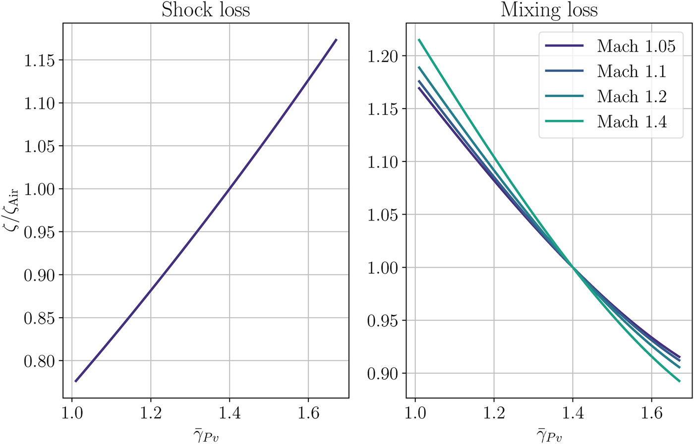
Recent investigations on flows of fluids of varying molecular complexity in transonic and supersonic blade rows (Baumgärtner et al., 2020a) highlighted that the wake mixing process and the associated loss are largely affected by the
in which
The right plot of Figure 1 shows the trend of the mixing losses as a function of the average isentropic pressure volume exponent. Higher efficiency penalties due to wake-mixing occur in mixing processes of fluids made by complex molecules and in thermodynamic states of the fluid for which
The results shown thus far point out that any loss correlation developed for ideal gas flows should be adapted to compute losses and efficiency trends of radial turbines operating with working fluids in nonideal thermodynamic states by, at least, introducing suitable values of
Turbine design methodology
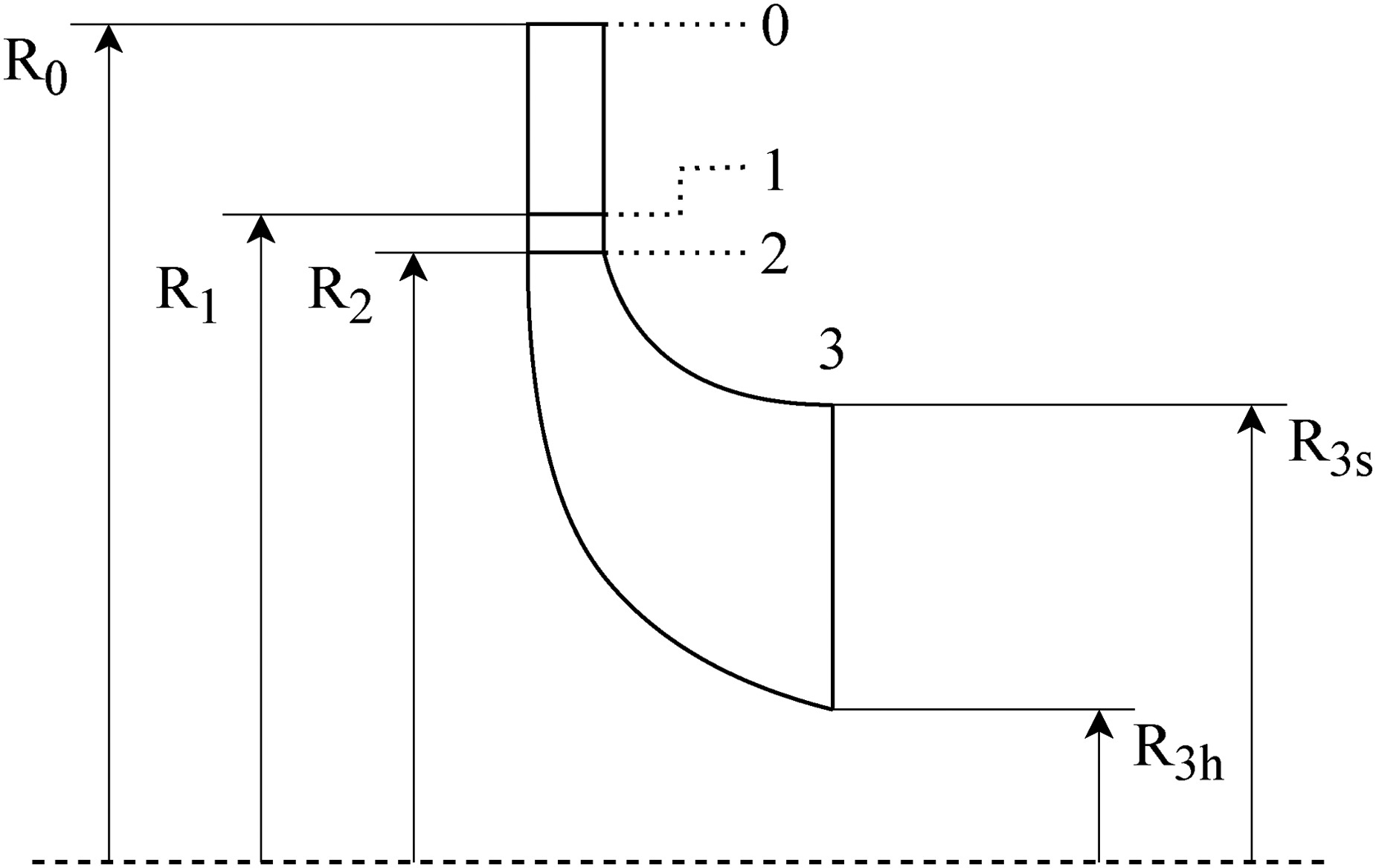
The turbomachinery design program TurboSim developed in this work is a reduced-order model (ROM) based on a quasi-3D calculation method of the flow passing through a radial-inflow turbine stage, composed by a stator and an impeller. The flow quantities and the main machine dimensions are evaluated at four sections in the stream-wise direction along the flow path, i.e., at the inlet and outlet of each blade row, as depicted in Figure 2. However, as opposed to a conventional lumped parameters approach, the flow quantities at each section are also calculated at an arbitrary number of locations along the span, to take three-dimensional effects into account. The most relevant 3D flow distribution, e.g. free- or controlled-vortex, can be imposed at the impeller outlet section to optimize the stage performance. The numerical framework is programmed in Python, and coupled to the thermodynamic libraries of the REFPROP software (Huber et al., 2022).
Figure 2.
Meridional view of a radial-inflow turbine stage with all the relevant dimensions indicated.
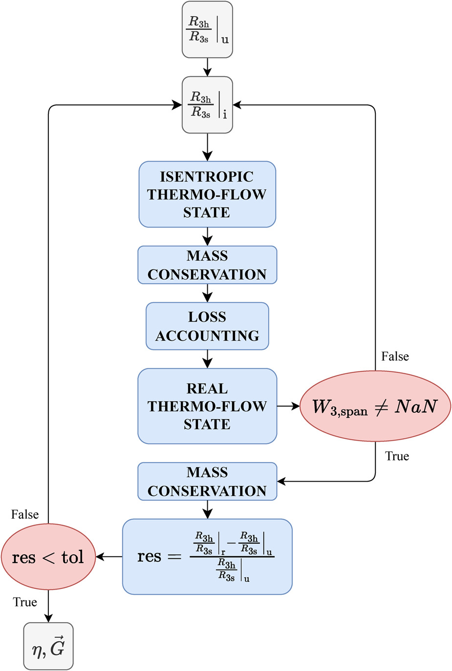
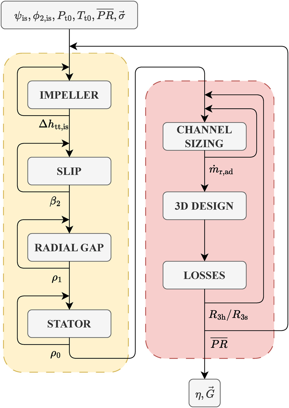
A simplified workflow illustrating the design methodology implemented in TurboSim is shown in Figure 3. The design is performed in two main steps, highlighted in the figure by means of the colored boxes. With reference to the yellow box, the stage is first sized by assuming isentropic and uniform flow along the span; the actual flow quantities at each span-wise location are subsequently calculated by selecting a span-wise flow distribution and by applying a loss model (red box). The whole design process is iterative, with several internal loops highlighted in the figure by the arrow wrapping around each block of the diagram. Convergence is achieved when the calculated mass-flow averaged pressure ratio
Impeller
The impeller is sized according to the classical method based on the work and flow coefficients (Chen and Baines, 1994). Given
where the isentropic enthalpy drop
Using the impeller design variables
Rearranging Equation 8 into Equation 9 yields the value of
The prediction of the optimal impeller incidence angle is based on the method proposed by Chen and Baines (1994). The impeller blade count is computed according to an empirical model (Glassman, 1976), see Equation 10, rigorously valid only for radial bladed impellers.
Given the blade count N and the isentropic tangential velocity
In Equation 11,
Given that the blade count N is a function of the impeller inlet absolute flow angle
Note that, as opposed to common design practices for radial-inflow turbines, the design methodology described here can lead to impellers characterized by non-zero blade sweep angles at the inlet. As impellers of supersonic ORC radial turbines operate at temperatures not exceeding 250–300 °C and feature relatively low peripheral speed, thus comparatively low thermo-mechanical stresses, sweep angles up to 45° can be adopted.
Radial gap
The flow quantities at the outlet of the stator vane are determined by assuming that the flow distribution follows a free vortex law in the radial gap. Two further design variables, namely the radial gap span ratio
The system of non-linear equations is solved by iterating on the density
Radial stator
The flow quantities at the inlet of the radial vane are calculated by specifying the value of the absolute inlet flow angle
and the energy balance
are iteratively solved to find the inlet flow velocity and the fluid thermodynamic properties.
Calculation of turbine efficiency
The total-total turbine efficiency is computed according to
where the term
Loss accounting
Stator passage loss
As radial vanes of supersonic RITs are typically constituted by prismatic blades featuring converging-diverging nozzle profiles, secondary flow losses are often negligible with respect to boundary layer losses occurring on the blades and on the endwalls. The model of Meitner and Glassman (1983) based on the two-dimensional boundary layer theory was adopted for the computation of blade profile losses
as also recommended in Manfredi et al. (2021).
In Equation 20, E is the energy factor and H the shape factor of the boundary layer, calculated as suggested by Meitner and Glassman (1983). The angle
that depends on the outlet flow conditions, where
where
Following Denton (1993), the entropy generation due to endwall loss is obtained by numerical integration of the right hand side term of
In the equation,
Mixing loss
Losses generated by wake mixing downstream of stator vanes and impeller blades are computed using the method documented in Denton (1993), in which the effective base pressure coefficient is computed as
Equation 24 is a generalization of the base pressure coefficient model to compressible flows and arbitrary working fluids (Baumgärtner et al., 2020a). In the equation,
in which
Shock loss
The entropy generation across shock waves formed at the trailing edge of either stator vanes and impeller blades is computed using the model based on first-principles documented in (Vimercati et al., 2018) and (Giuffre’ and Pini, 2021). The governing equations are the Rankine-Hugoniot (RH) relations for an oblique shock, reported by Equation 26–29.
where
The entropy change across the shock is equal to
where
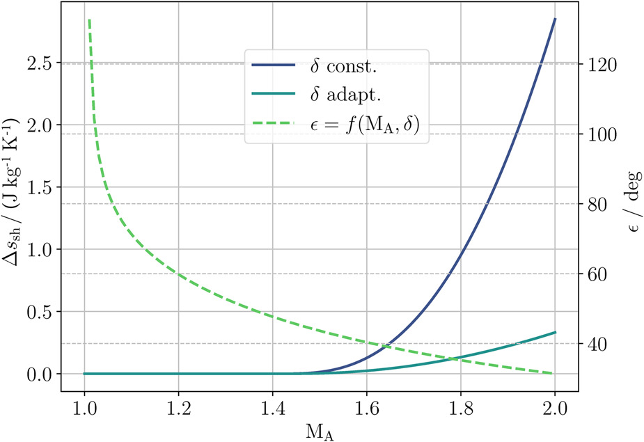
To assess the sensitivity of the shock losses to different pre-shock conditions and shock-wave angle, the entropy generation across an oblique shock wave inclined at 45° has been computed as a function of the pre-shock Mach number
Figure 4.
On the left y-axis: entropy change obtained by solving the RH governing equations (solid lines) as a function of the pre-shock Mach number M A ε = 45 ∘ M A ε M A
The accuracy of the first-principle shock loss model has been verified against results from a two-dimensional CFD simulation. Table 1 reports the comparison of the computed entropy change with the two models for a case of supersonic nozzle flow passing through a normal shock, highlighting that the results between the two models are very similar.
Radial gap loss
Losses in the radial gap are attributed to viscous friction on the endwalls and the associated entropy generation can be expressed as (Whitfield and Baines, 1990)
where
in which the turbulent friction coefficient
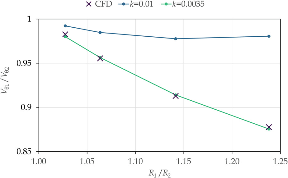
Equation 33 is solved in combination with 14 and 16 to find the flow state at the outlet of the radial gap. A value
Figure 5.
Variation of the tangential velocity ratio as given by Equation 33 for two values of k (solid lines) and comparison with CFD results (×).
Impeller loss
Loss sources in the impeller are assumed to be predominantly related to passage and tip leakage flow. Passage flow losses are due to viscous dissipation in the boundary layers, and to mixing of the passage vortex. The semi-empirical model proposed by Baines (1998), accounting for viscous, blade loading and secondary flow losses, is used in this work to compute the passage losses. The model, reported in Equation 35, has been shown to be more accurate of that of Rodgers documented in Whitfield and Baines (1990) for predicting the efficiency of supersonic ORC RITs by Manfredi et al. (2021).
In Equation 35, c is the blade chord, z the impeller axial length,
Losses due to tip leakage flow are computed in accordance to Baines (1998)
In Equation 36,
Diffuser loss
The losses occurring within the diffuser, assumed to be of conical shape, are computed by resorting to the model proposed by Agromayor et al. (2019). The governing equations are formulated as an implicit system of ordinary differential equations that are solved iteratively. The diffuser cant angle, the wall semi-aperture angle and the diffuser area ratio are specified as inputs, as well as the geometry and the flow state at the exit section of the impeller. Viscous flow losses in the diffuser are computed by specifying the friction factor. In this work this was fixed to
Model verification
In order to verify the accuracy of TurboSim, the results of the model have been compared with those obtained from CFD simulations. Two radial-inflow turbine test cases have been considered. The first test case consists of a high-pressure ratio RIT used as gas generator in the T100 turbo-shaft engine, designed and tested by Sundstrand Power Systems (Jones, 1996). The second test case is the so-called ORCHID turbine, representative of an ultra-high pressure ratio, single stage RIT for experimental research on high temperature ORC systems. The stage has been designed and optimized by means of high-fidelity CFD methods by De Servi et al. (2019).
CFD setup
The three-dimensional geometry of the T100 was constructed based on data from the open literature (Sauret, 2012) and the discretization of the three-dimensional geometry was performed using a commercial software (Ansys® CFX, n.d.). Unsteady, single-passage, RANS computations were used to predict the turbine performance, using a structured mesh comprising about 3 million cells. The optimal cell count of the stator, impeller, and diffuser was informed from a mesh sensitivity study (Matabuena, 2023) based on the Richardson extrapolation method (Roache, 1998). For the ORCHID turbine, a mesh of approximately 4 million cells was used to discretize the computational domain, as suggested in Cappiello et al. (2022). In this case, the computational domain only comprised the mesh of the convergent-divergent vane and that of the impeller.
For both test cases, the Ansys® CFX (n.d.) flow solver was employed. The discretization of the advection terms was performed using a central differencing scheme (CDS), ensuring a second order accurate solution. Turbulence closure was obtained through the Shear Stress Transport (SST
Table 2.
Boundary conditions and fluid models used in the uRANS simulations.
| T100 | ORCHID | |
|---|---|---|
| Air | MM | |
| Ideal-gas | MEoS | |
| 1.4 | 1.025 | |
| 4.13 | 18.1 | |
| 477.6 | 573 | |
| 1.0 | 0.738 | |
| 1.4 | 0.952 | |
| 0.724 | 0.443 | |
| 71700 | 98119 |
[i] The thermodynamic conditions of the MM fluid have been computed using a look-up table (LUT) method. The LUT has been generated using the multi-parameter equation of state (MEoS) (Span and Wagner, 1996) implemented by Huber et al. (2022).
Performance comparison
Table 3 reports the predictions of the turbine power and total-total efficiency obtained with TurboSim and with the CFD. The deviation in the efficiency values is within 1% for both cases. For the T100, the experimentally measured efficiency (Jones, 1996) is also reported. It can be observed that the CFD over-predicts the efficiency by 4%. A possible cause of discrepancy is due to the choice of not modeling the losses associated to the leakage flow from the hub.
Table 3.
Turbine performance prediction obtained with the ROM, CFD and experiments.
| T100a | ORCHID | ||||
|---|---|---|---|---|---|
| Quantity | ROM | CFD | Exp. | ROM | CFD |
| 66.3 | 69.8 | 10.1 | 10.2 | ||
| 91.2 | 92.1 | 87.1 | 84.9 | 85 | |
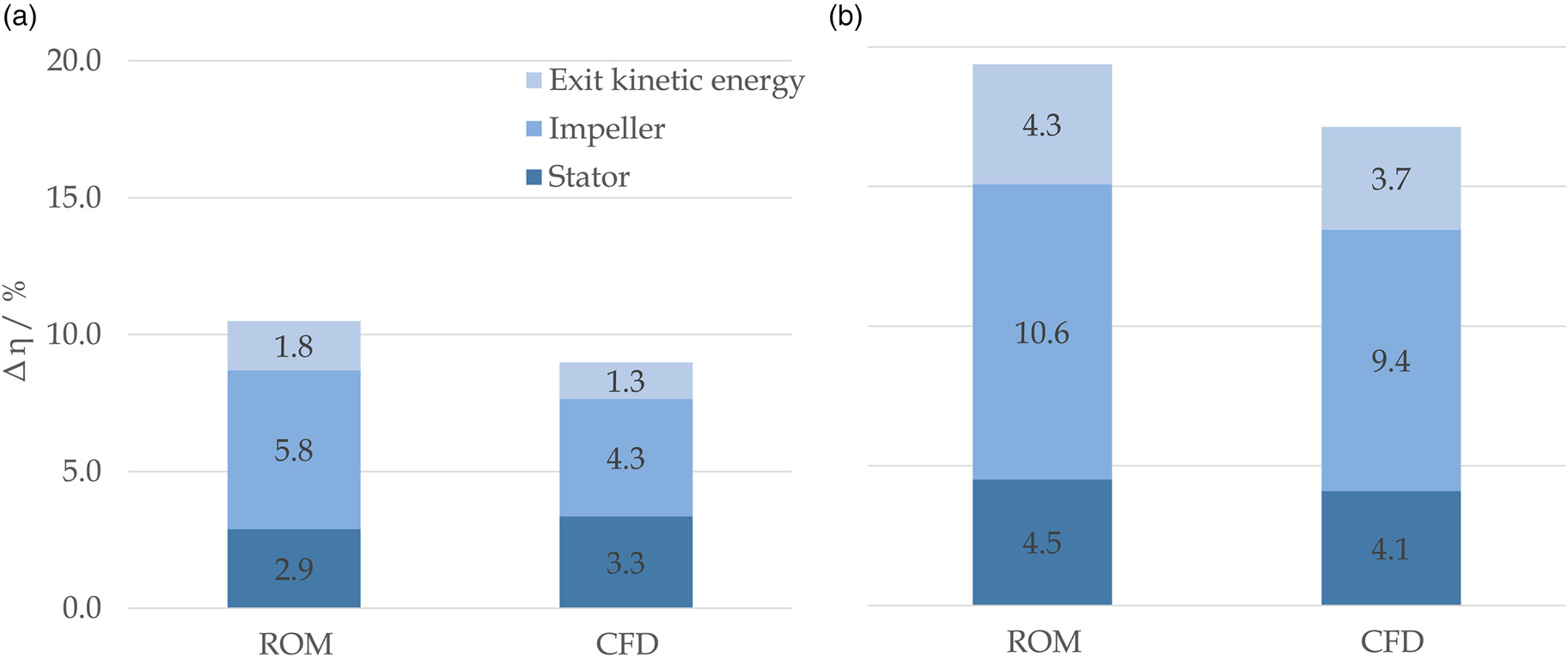
Further insights on the accuracy of the loss accounting methodology implemented can be gained by performing a loss breakdown analysis. The CFD-based loss breakdown was performed by mass-flow averaging the flow quantities at the inlet and outlet of each component in both time and space as
where q is a generic time and space dependent thermo-physical quantity,
By applying Equation 38 to calculate the space-time averaged isentropic outlet temperature and the entropy change across each component, the efficiency deficit can be calculated as
where
Figure 6a and 6b show the results of the loss breakdown analysis performed with the two models. The efficiency penalty across the stator and the impeller are displayed, along with the loss associated to the exit kinetic energy. The outcome of the loss breakdown analysis qualitatively shows that TurboSim predicts efficiency values close to those of the CFD. Notably, the ROM successfully captures the lower efficiency of the ORCHID turbine, which is characterized by a comparatively much higher pressure ratio. Minor deviations between the two models arise when comparing the share of loss of each turbine component, especially concerning the impeller losses which are overestimated by the ROM. In spite of the differences in the results illustrated in the plot, the accuracy of TurboSim is deemed adequate for systematic studies aimed at establishing guidelines for the design of hiTORC-RIT.
Results
TurboSim is used to generate design maps, namely contours and charts of key performance metrics as function of the most relevant independent variables of Equation 3. In particular, the influence of
where
This relation was used to compute the mass flow rate
It should be noted that
Influence of the working fluid and γ ¯ P v
The influence of the working fluid and
Figure 7.
Total-static efficiency of RITs as a function of γ ¯ P v M C S P = 0.025 m V R = 6 , 20 and 80 ψ i s 0.7 1.0 1.3 ϕ 2 , i s 0.4 ± 1 %
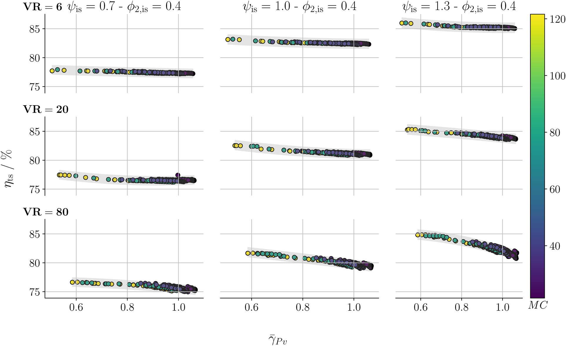
Table 4.
Fluids used to generate the data displayed in Figure 7 and their main characteristics.
| Fluid name | Chemical name | ||
|---|---|---|---|
| Ethanol | Ethyl alcohol | 21.51 | 1.080 |
| Butane | n-Butane | 29.53 | 1.054 |
| Pentane | – | 39.80 | 1.040 |
| MM | Hexamethyldisiloxane | 78.35 | 1.026 |
| Dodecane | – | 121.63 | 1.018 |
The plots show that the efficiency decreases as the value of
To better display the role of
Table 5.
Boundary conditions for the turbine operating with the LMC and the HMC (siloxane MM) fluid.
| LMC | 7.0 | 0.2 | 4.0 | 1.0 | 1.15 |
| MMi | 78.35 | 0.2 | 1.1 | 0.95 | 1.0 |
| MMni1 | 78.35 | 1.0 | 1.1 | 0.71 | 0.92 |
| MMni2 | 78.35 | 2.0 | 1.1 | 0.43 | 0.78 |
Figure 8.
Reduced P − T γ P v V R = 20 ( □ ) ( ◯ ) ( Δ )
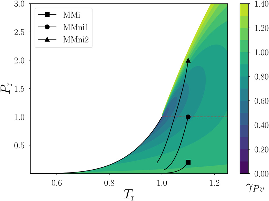
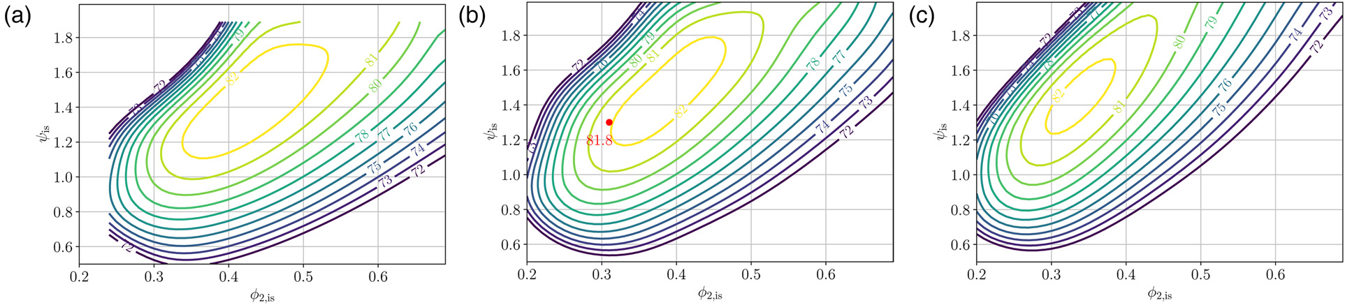
Figure 9.
Total-total ( ◯ ) ( Δ ) ψ i s V R ϕ 2 , i s = 0.4 γ ¯ P v
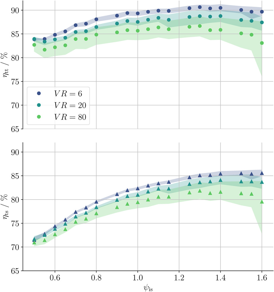
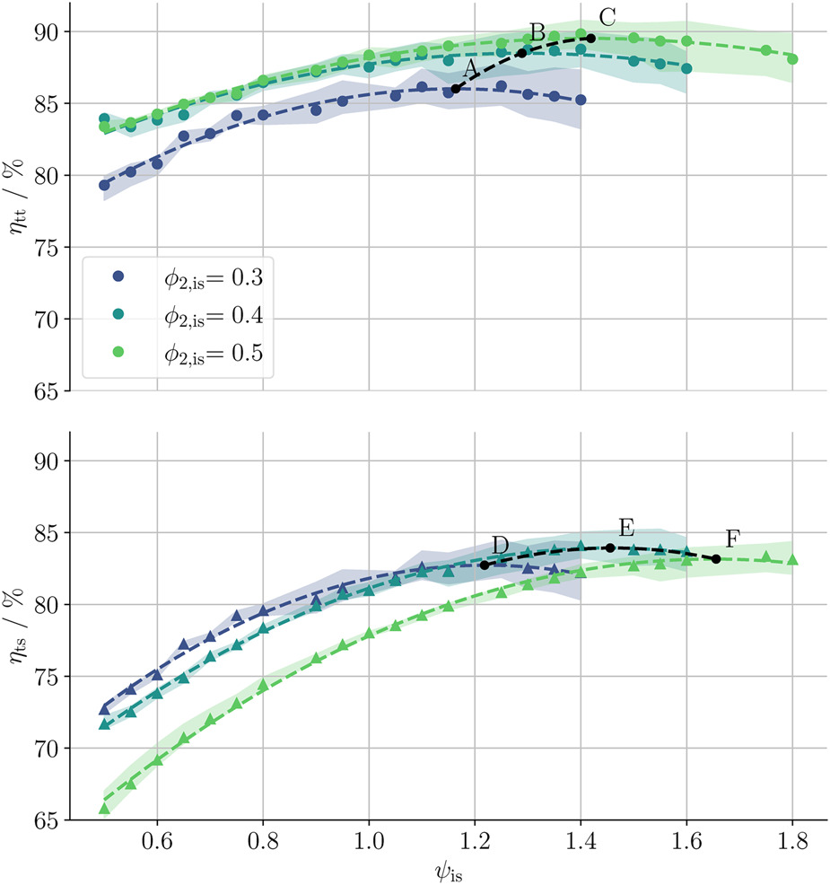
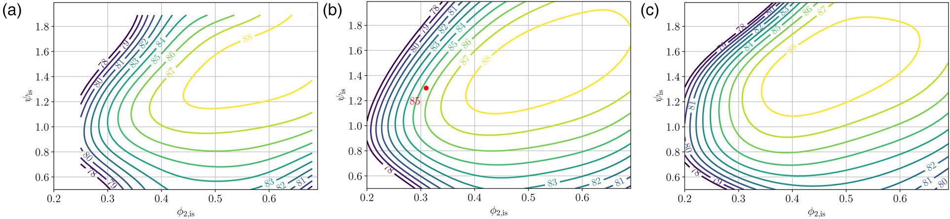
Figure 10.
Total-total ( ◯ ) ( Δ ) ψ i s ϕ 2 , i s V R = 20 γ ¯ P v ϕ 2 , i s 2 n d 2 n d ψ i s ϕ 2 , i s
Loss breakdown analysis
Insight into the impact of the duty coefficients
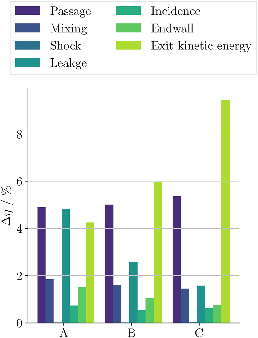
Figure 11.
(a) Meridional flow path of the optimal designs A, B and C of Figure 10. The axial and radial coordinates are non-dimensionalized by the tip radius of case B. (b) Impeller absolute flow angles ( α ) ( β )
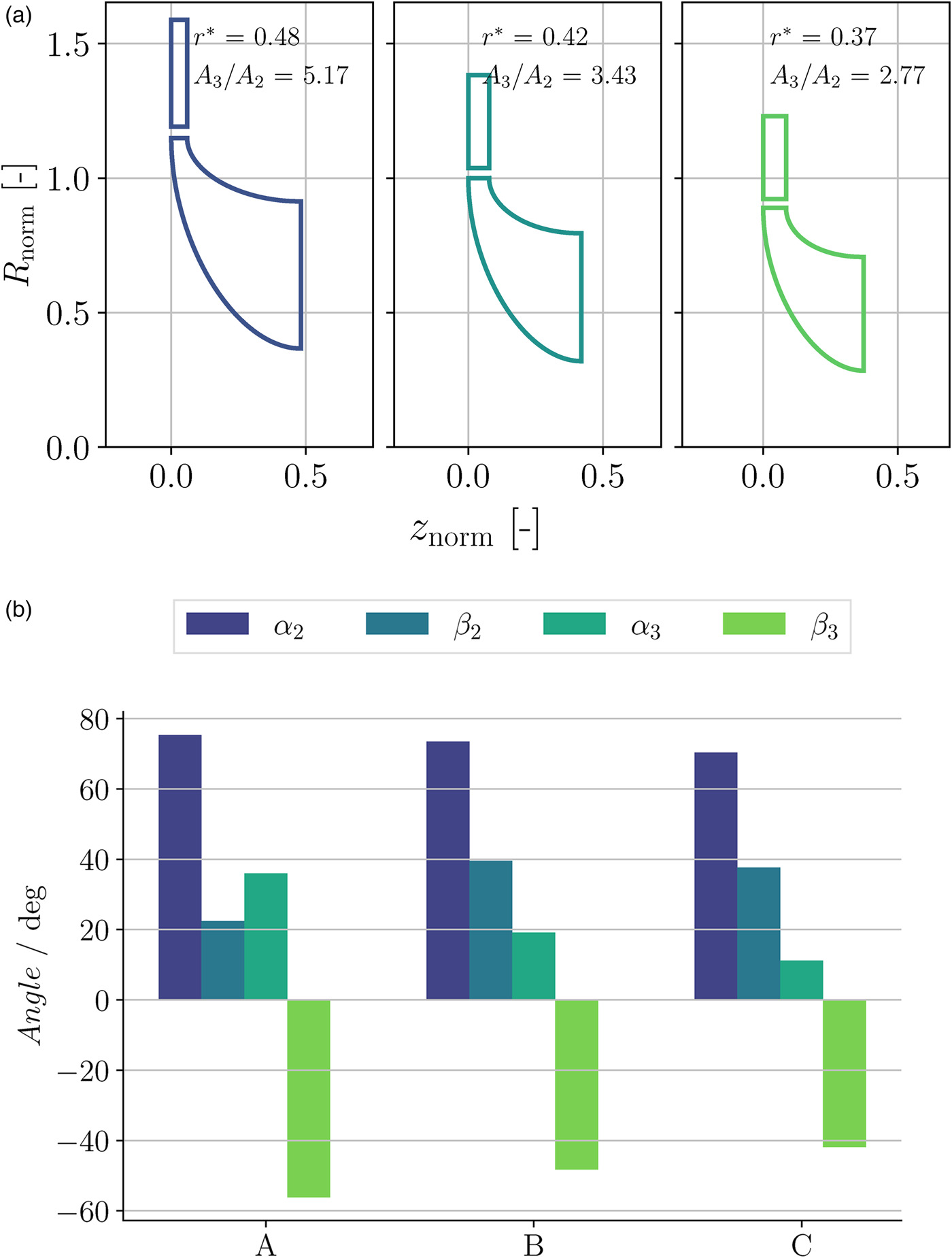
Figure 12.
Stage (stator + impeller) loss breakdown for optimum designs A, B and C shown in Figure 10. The optimal work coefficients are, respectively, 1.15 1.3 1.4 V R = 20
To further clarify the effect of
Figure 13.
Absolute Mach number at the outlet of the stator ( ◯ ) ( □ ) ψ i s V R = 20 S P = 0.025 m ϕ 2 , i s = 0.4
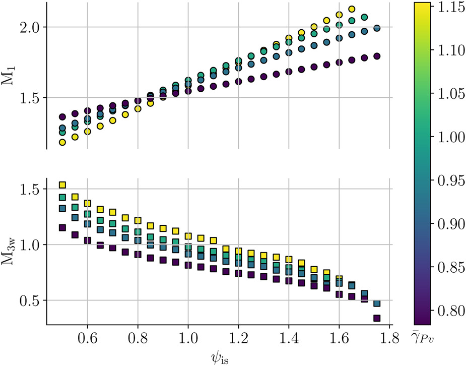
Figure 14.
Cumulative stator ( ◯ ) ( □ ) ψ i s V R = 20 S P = 0.025 m ϕ 2 , i s = 0.4
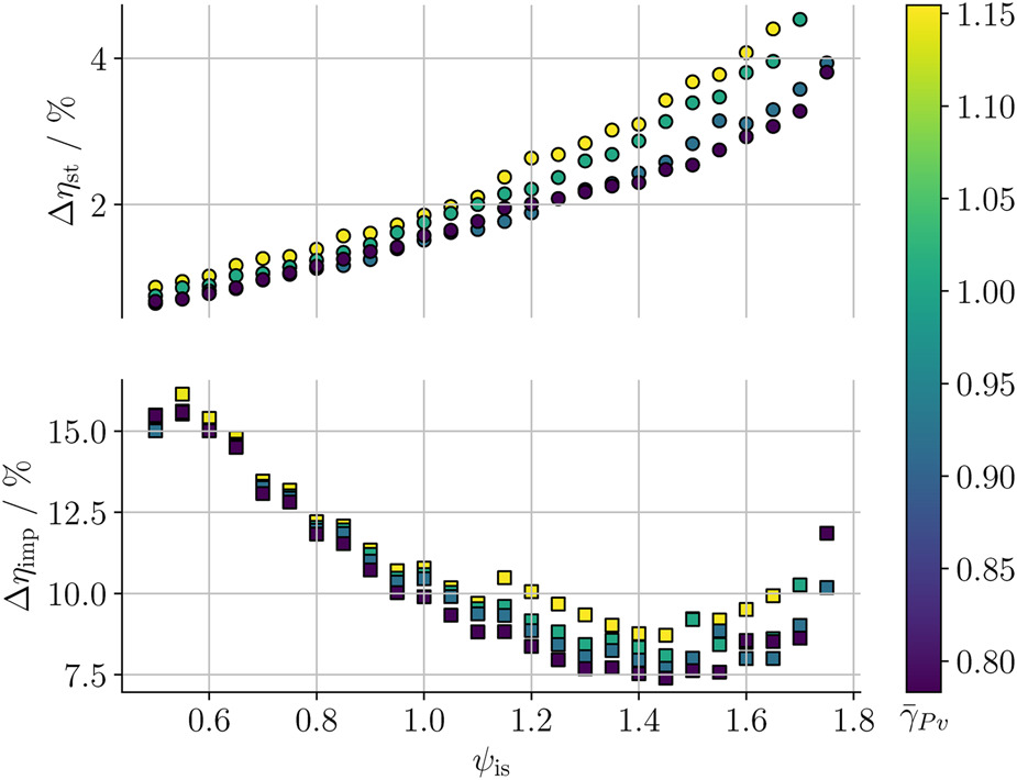
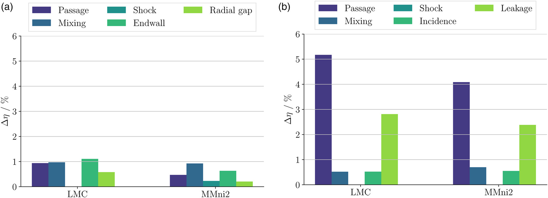
Figure 15 reports the results of the loss breakdown analysis for the stator and the impeller of two turbines designed for the cases LMC and MMni2, featuring
Figure 15.
Loss breakdown in the stator (a) and the impeller (b) for the LMC and MMni2 cases listed in Table 5. ψ i s = 1.35 ϕ 2 , i s = 0.4 V R = 20
Influence of the meridional velocity ratio on efficiency
A design parameter which largely affects the turbine layout and whose optimal value for hiTORC-RIT is not reported in the literature is the meridional velocity ratio of the impeller, herein denoted with
Design guidelines
The results that have been used to generate the maps are finally converted in design guidelines, namely charts that can be used to quickly size the turbine and compute its efficiency in system-level analysis and optimization. A relevant example in which such a model is exploited is reported in Krempus et al. (2023).
Figure 18 shows the trend of maximum
Figure 18.
Optimal ψ ϕ 2 ( Δ ) V R η t t η t s V R η t t η t s γ ¯ P v = 1.15 γ ¯ P v = 1.0 γ ¯ P v = 0.92 γ ¯ P v = 0.78
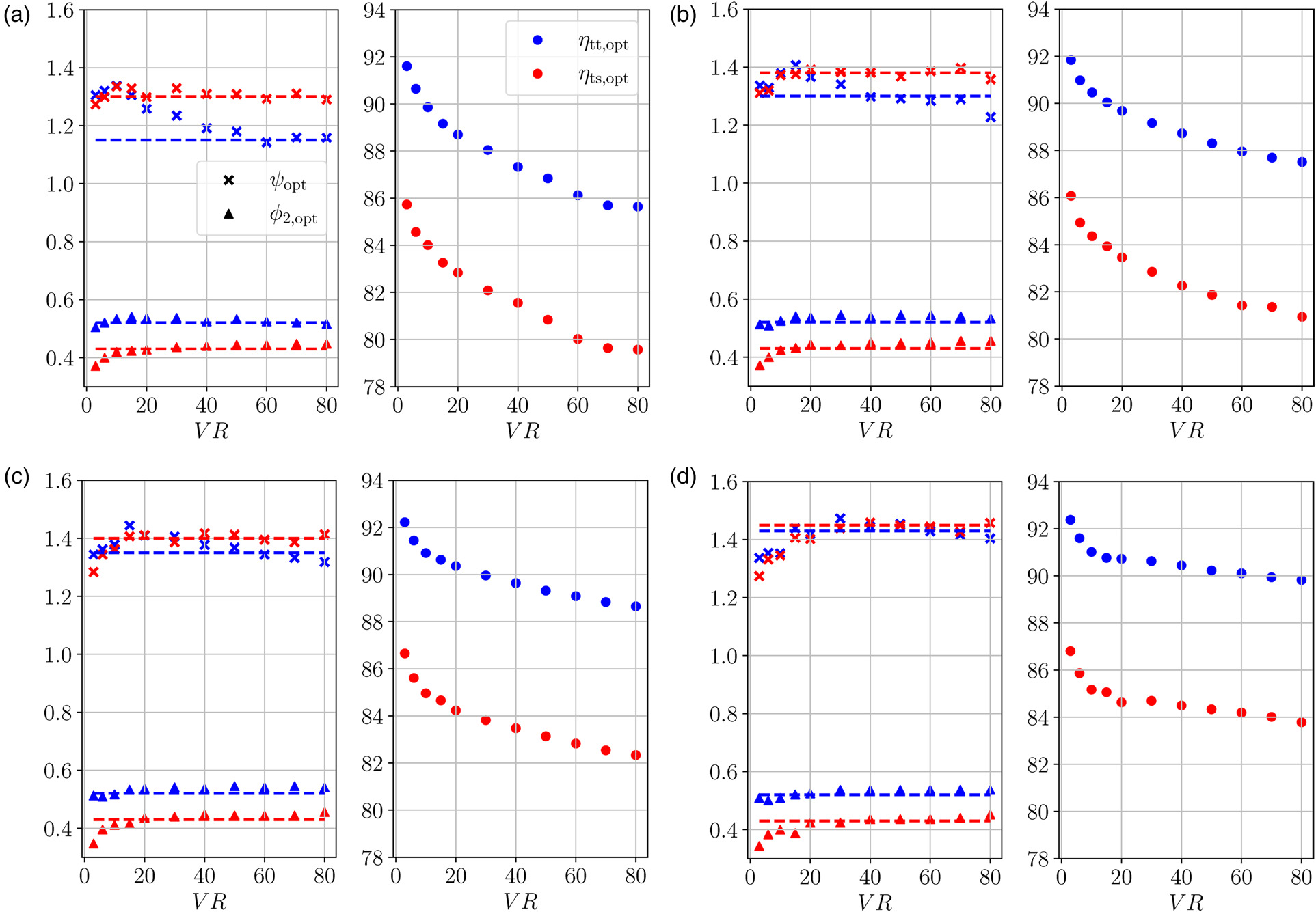
The optimal flow coefficient
On the contrary, the optimal load coefficient
A similar trend occurs with the value of
In summary, when designing RITs operating with fluids in thermodynamic states for which
Considering the values of efficiency, both the optimal
Conclusion
Design guidelines for radial-inflow turbines of high-temperature organic Rankine cycle power systems are documented. The influence of the working fluid, nonideal thermodynamic effects, and of the volumetric flow ratio on the choice of optimal design parameters
The efficiency predicted by the reduced-order model is within 1% the value obtained with uRANS. The model was able to correctly capture the effect of the volumetric flow ratio on the efficiency.
The optimal value of duty coefficients
The values of the optimal duty coefficients derived in this work differ from those that can be inferred from the design maps of Rodgers (1987) and Chen and Baines (1994). Therefore, it can be argued that the application of conventional design maps can lead to sub-optimal hiTORC-RIT designs.
Nonideal thermodynamic effects quantified through
The results documented in this work extend the analysis provided in (Perdichizzi and Lozza, 1987; Da Lio, 2019; Manfredi et al., 2023) to volumetric flow ratios beyond 50. Similar conclusions related to the choice of the optimal load coefficient presented in (Da Lio, 2019) were found.
The study offers new insights into why hiTORC-RIT operating in nonideal thermodynamic conditions can achieve relatively high efficiency, even when designed for very high volumetric flow ratio.