
Introduction
Modern turbomachinery design highly relies on computational fluid dynamics(CFD) for analyzing its performance by solving the steady and unsteady Euler equations or Reynolds-averaged Navier-Stokes(RANS) equations. In numerical analysis, the robustness and the convergence rate of involved solution methods are vitally important for design engineers, as they largely dictate the accomplishment of a design task. Typically, there are two kinds of numerical methods for pseudo-time integration: explicit methods and implicit methods. The representative explicit methods are the multi-stage Runge-Kutta methods (Jameson et al., 1981). Their advantages lie in the low memory consumption, low CPU cost per iteration, and easy implementation. Because of this, they have been very popular in the CFD community. The biggest disadvantage of the explicit methods is their conditional stability. To achieve a stable solution, the time step is limited by the Courant-Fredrichs-Levy(CFL) stability condition. This time step limit is manifested by flow field analysis at off-design conditions and harmonic balance analysis with a large maximum grid-reduced frequency (Hall et al., 2013).
The implicit methods, on the other hand, often have higher memory consumption and higher CPU cost per iteration, and are much more difficult to implement, when compared with the explicit methods. The biggest advantage of the implicit methods is better stability. Thus a much bigger time step can be allowed in an analysis leading to reduced overall time cost. The extended stability of an implicit method depends on the approximation of the system Jacobian matrix. A better approximation generally leads to higher stability but incurs more implementation complexity and computing resources.
The Lower-Upper Symmetric Gauss-Seidel(LU-SGS) method is a popular implicit method, as it represents a good compromise between the advantages and the disadvantages of implicit methods. In a steady analysis, its maximum allowable Courant number is theoretically infinite, though anything more than 1,000 does not make any meaningful difference to the convergence rate of a solution. The LU-SGS method can also be used as a preconditioner for the Runge-Kutta schemes to achieve a better convergence rate and stability (Rossow, 2006).
When it comes to the harmonic balance equation system, the implementation of the LU-SGS method is quite difficult because solutions at different time instants are coupled. To reduce the programming complexity, the Jacobian matrix of the time spectral source term is excluded from the LU-SGS method and it is implicitly integrated using a block Jacobi(BJ) method (Wang and Huang, 2017). Although numerical experiments demonstrate that this decoupled implicit treatment of the time spectral source term can increase solution stability, a thorough stability analysis of this numerical method has not yet been reported in the open literature.
There are two main methods for assessing the stability and the convergence properties of a given numerical scheme. One is well known as the von Neumann method developed by Charney et al. (1950), which has been widely used to analyze the stability of a linear equation system with constant coefficients and periodic boundary conditions. A von Neumann analysis shows that the first-order forward temporal integration scheme is unconditionally unstable for the linearized Burger’s equation in the harmonic balance form when a first-order upwind scheme is used for the spatial discretization (Hall et al., 2013). However, the stability of an equation system can be impacted by inlet, outlet, slip wall boundary conditions, and so on. The effect of these boundary conditions on the stability of an equation system can only be analyzed by using the matrix or eigen-analysis method. The Laplace equation and a two-equation model hyperbolic system were examined using the matrix method with various boundary conditions and stretched grids (Roberts and Swanson, 2005). Eriksson and Rizzi (1985) investigated the solution behaviour of a center scheme for two-dimensional Euler equations. The beneficial effects of local time-step scaling and artificial dissipations were studied using an eigen-analysis.
This paper presents the stability analysis results of solution methods for steady and harmonic balance form Euler equations. The solution methods involve a central scheme with blended second- and fourth-order artificial dissipations for the spatial discretization and a Runge-Kutta scheme for pseudo-time integration. The LU-SGS method and LU-SGS/BJ method are used as the implicit residual smoothing for the steady and harmonic balance solutions, respectively. Both the von Neumann and the matrix methods are used to analyze the stability of the involved solution methods. Based on the stability analysis results, the impact of the boundary conditions and the block Jacobi method on solution stability and convergence rate can be analyzed, providing insights on how to obtain a solution fast and robustly. Though the stability analysis is carried out based on the two-dimensional Euler equations, the conclusions can be readily extended to the three-dimensional RANS equations as demonstrated by using a Laval nozzle and the NASA rotor 37.
Methodology
Flow governing equations
The unsteady Euler equations for an ideal gas in a two-dimensional Cartesian coordinate system have been used in the investigation. They are written in a conservative and differential form as
whereTo simplify the following presentation, Equation (1) is rewritten as the following semi-discrete form
whereHarmonic balance method
The harmonic balance method is a computationally efficient reduced-order technique for time-periodic flows within turbomachinery (Hall et al., 2002). Its analysis time cost can be 1-2 orders of magnitude lower compared with the dual time-stepping method using a whole annulus computational domain for turbomachinery applications. With the harmonic balance method, the time-dependent flow variables are approximated using a truncated temporal Fourier series
where
where
and
(5)
Accordingly the time derivative term of the conservative variable vectors at
where
(7)
The matrix
The pseudo-time derivative term is introduced to facilitate the use of time-marching methods to solve the harmonic balance equations.
Runge-Kutta scheme and LU-SGS method
The time integration is accomplished through a classic four-stage Runge-Kutta scheme together with the LU-SGS method. The LU-SGS method was first proposed by Yoon and Jameson (1988) as a time integration method. It was later used as a residual smoother at each stage of a Runge-Kutta scheme to improve stability and convergence rate (Rossow, 2006). The solution update at the
where
While the explicit scheme is conditionally stable, the stability and convergence rate of the solution can be further improved by employing the implicit method, the LU-SGS method, as a preconditioner of the Runge-Kutta method. Subsequently, the solution increment is obtained by solving the following equations
where
here
where matrices
where
in which
More details about the derivation of the operators
So far the Jacobian matrix of the time spectral source term is not included on the left-hand side of Equation (11), implying that the time spectral source term is integrated explicitly. As the maximum grid-reduced frequency becomes high, the maximum allowable Courant number will be limited or even solution instability can occur in the harmonic balance equation system.
Block Jacobi method
To mitigate the impaired solution stability caused by the time spectral source term, it needs to be integrated implicitly together with other terms as follows
However, the exact inversion of the system Jacobian matrix of
where M is the number of block Jacobi iterations and the initial solution increment
When using the LU-SGS/BJ method to solve the harmonic balance equation system, it is crucial to consider the influence of the time spectral source term in scalar B. Otherwise, the full potential of the LU-SGS/BJ method cannot be exploited. The scalar B can be modified as follows
where
Boundary conditions
In general, there are four kinds of boundary conditions used in this numerical analysis: subsonic inlet, subsonic outlet, slip wall, and periodic boundary conditions. At a subsonic inlet, the total pressure, total temperature, and flow angle are specified, while the static pressure is extrapolated from the interior domain to the boundary. Additionally, one can also extrapolate the one-dimensional Riemann invariant to the inlet boundary. The Riemann invariant
where V is the velocity magnitude and c is the speed of sound.
The well-posedness of a boundary condition is important for a numerical analysis as it can affect solution convergence characteristics and even solution accuracy. Extrapolating the Riemann invariation at an inlet boundary has been found to offer better convergence properties for nozzle flows (Jameson and Caughey, 2001). Nevertheless, there is currently a lack of stability analysis supporting this conclusion. This paper will examine the better convergence characteristics of extrapolating the Riemann invariant through stability analysis.
At a subsonic outlet boundary, the static pressure is specified, while the density and momentum in the x and y directions are extrapolated from the interior domain to the boundary. To obtain a meaningful unsteady solution for a Laval nozzle and the NASA rotor 37, a sinusoidal static pressure at the outlet is prescribed
where
von Neumann method
Though Swanson et al. (2007) performed a stability analysis of the RK/LU-SGS methods for two-dimensional steady Euler equations, there has been no such effort of the RK/LU-SGS methods for solving the harmonic balance equation system in the open literature. The stability and damping behaviours of the RK/LU-SGS methods will change dramatically due to the time spectral source term in the harmonic balance equation system. To improve the solution stability of a harmonic balance equation system, the block Jacobi method is often used. Therefore, there is also a need to perform a stability analysis of the RK/LU-SGS/BJ method for solving the harmonic balance equation system.
In the von Neumann analysis, we assume the Euler equations are solved in a finite domain with periodic boundary conditions. Let us define a Cartesian grid consisting of
where
The numerical error
where
As the Cartesian grid is uniform,
where
in which
Substitute a single spatial harmonic
where
where
and
Through M Jacobian iterations, the transformed increment of the solution can be simplified as
where
which can be obtained as follows
in which the initial value
When
where the amplification matrix
in which
Typically, the Fourier symbol
Matrix method
The matrix method, also known as the eigenvalue analysis, is a more general approach to stability analysis. It allows for considering various boundary conditions, grid nonuniformities and flow field nonuniformities. In the case of a non-uniform mesh, the total residual function
(26)
where the convective fluxes through a bounding surface with the index
Fluxes at a bounding surface are calculated by simply averaging their values on two sides of the bounding surface. For example,
where
In the stability analysis based on the matrix method, the solution iteration needs to be written in a matrix form. For an explicit scheme, the solution increment is given by
where the index
(30)
where
where
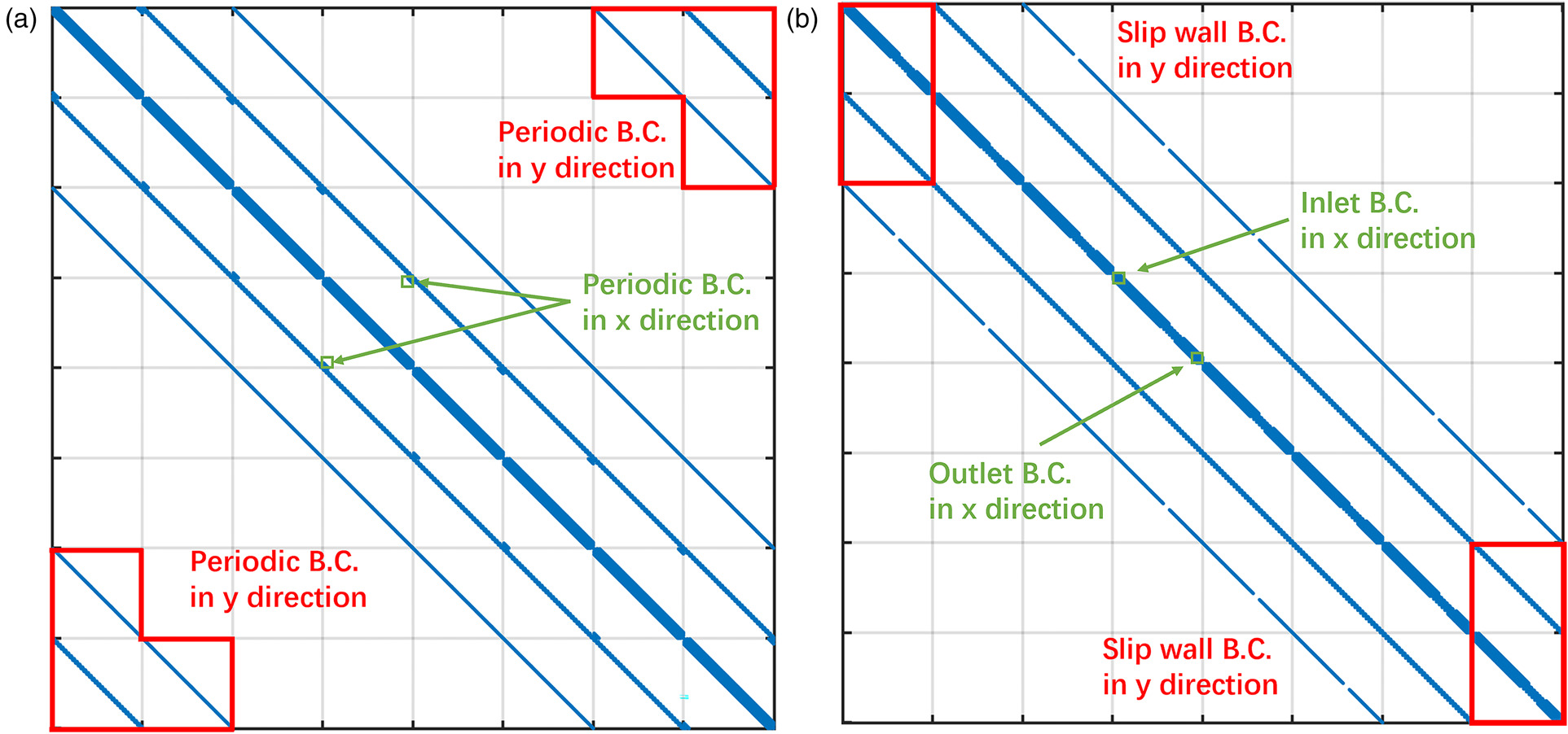
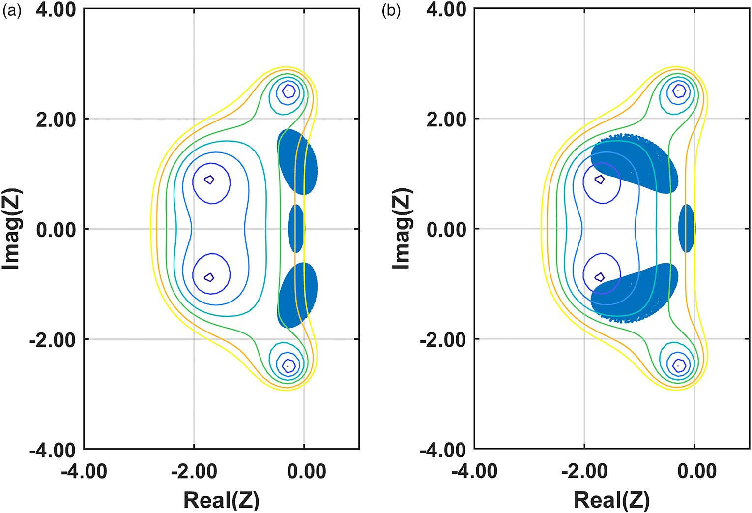
Firstly, the periodic boundary conditions in the x and y directions are applied in the matrix method, as illustrated in Figure 1a. The use of periodic boundary conditions in the y direction introduces non-zero off-diagonal elements to the system Jacobian matrix
Figure 1.
Visualization of the Jacobian matrix of the spatial discrete operator for the 2-D Euler equation system. Nonzero elements are displayed as filled blue dots. (a) Periodic B.C. in x and y directions. (b) Inlet,outlet B.C. in x direction and slip wall B.C. in y direction.
The Jacobian matrix
where
where
In the matrix method, if the spectral radius of
Results and discussion
This section presents two different parts. The first part is aimed at investigating the stability of the combination of explicit Runge-Kutta methods with the JST scheme for solving steady and time spectral form Euler equations by using the von Neumann method and the matrix method. The impact of various boundary conditions on solution stability is considered by the matrix method. The second part focuses on the stability analysis of the LU-SGS method for solving the time spectral form 2-D Euler equations and also the stabilization of the block Jacobi method for different grid-reduced frequencies.
The stability of an explicit Runge-Kutta scheme with different boundary conditions
First, the stability of an explicit Runge-Kutta scheme for solving steady Euler equations with periodic boundary conditions is examined using both the von Neumann method and the matrix method. The computational domain has a length of 0.2 meters and a height of 0.08 meters as shown in Figure 2. It is discretized using a uniform Cartesian grid with 33 points in the x direction and 9 points in the y direction. The resulting grid aspect ratio is

Figure 3.
The locus of the Fourier symbol and the eigenvalue spectrum of the transform matrix with periodic boundary conditions, uniform flow fields and grids ( AR = 0.625 , Ma = 0.5 , β = 0 ∘ , k ( 4 ) = 0.21 , σ = 3 )
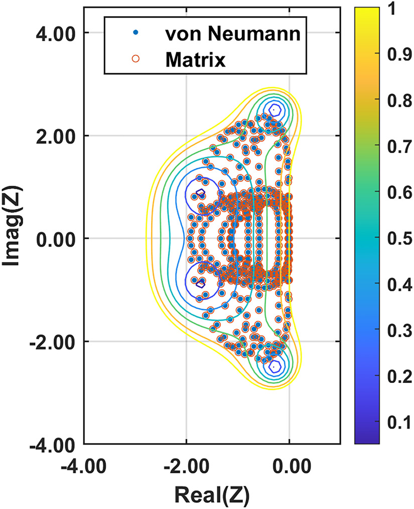
The locus of the Fourier symbol
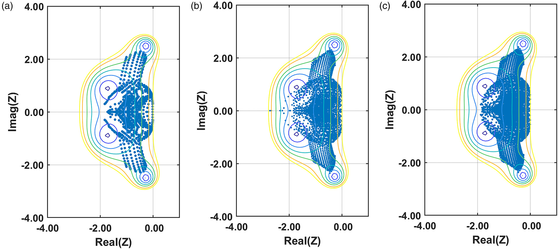
To assess the impact of various boundary conditions by the matrix method, these boundary conditions are categorized into four combinations. The first combination serves as a reference, which includes periodic boundary conditions in the x and y directions. The second combination involves inlet and outlet boundary conditions in the x direction and periodic boundary conditions in the y direction. The third combination includes wall boundary conditions in the y direction and periodic boundary conditions in the x directions; The fourth combination consists of inlet and outlet boundary conditions in the x direction and wall boundary conditions in the y direction. The eigenvalue spectra of these four combinations of boundary conditions are presented in Figure 4.
Figure 4.
The eigenvalue spectra of the transform matrix for various boundary conditions. ( k ( 4 ) = 0.021 , σ = 3 )
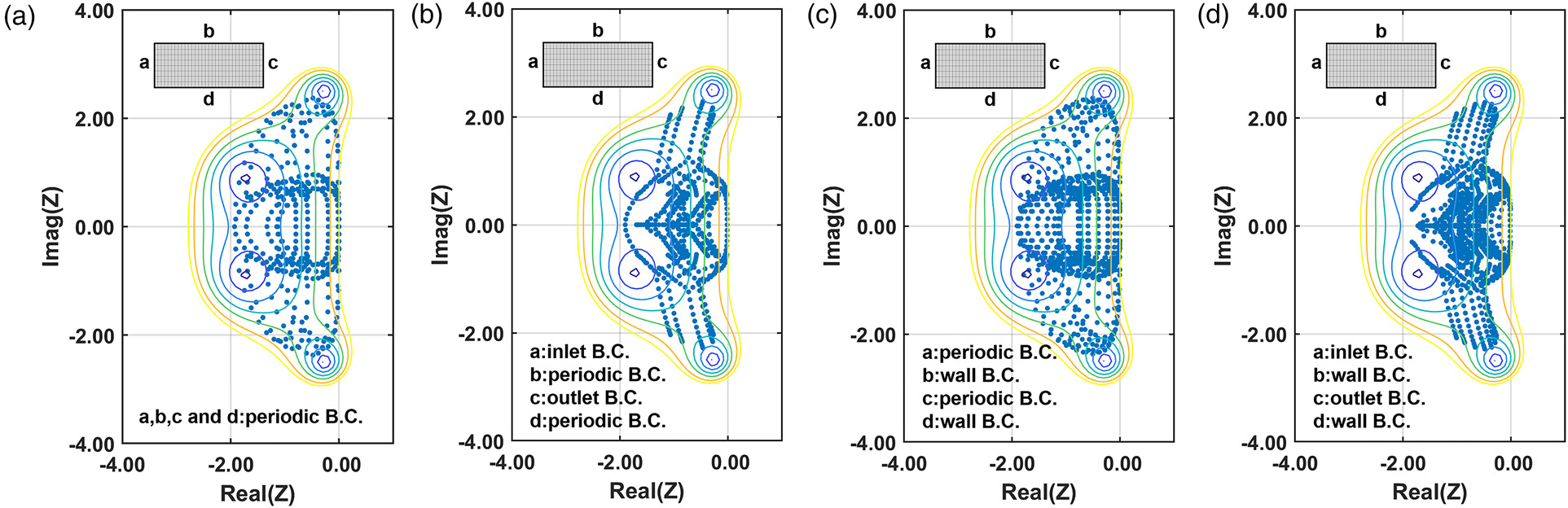
Comparing Figure 4a and b, it can be seen that the inlet and outlet boundary conditions change the distribution of the eigenvalues considerably in the complex plane. Figure 4c presents the eigenvalue spectrum of the third combination, which is quite similar to that in Figure 4a. It implies that the impact of the wall boundary conditions is smaller than that of the inlet and outlet boundary conditions. Figure 4d presents the eigenvalue distribution of the fourth combination, which resembles that of the second one. In conclusion, different combinations of boundary conditions result in varying distributions of eigenvalues in the complex plane, leading to different stability and damping properties. Among these boundary conditions, inlet and outlet boundary conditions have the most significant impact on the eigenvalue spectrum, leading to enhanced stability. Note the impact of boundary conditions diminishes with the increase of grid points.
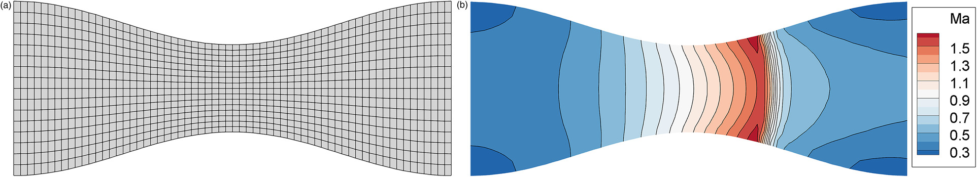
Next, the impact of different baseline flow fields and inlet boundary conditions on solution stability is investigated by the matrix method. The stability analysis is performed on a Laval nozzle as shown in Figure 5a. A mesh with 65 grid points in the x direction and 17 grid points in the y direction is used to discretize the domain. At the inlet, the total pressure
Figure 5.
The computational mesh and Mach number contours within a Laval nozzle obtained from solving the 2-D steady Euler equations. (a) mesh. (b) Mach number contour.
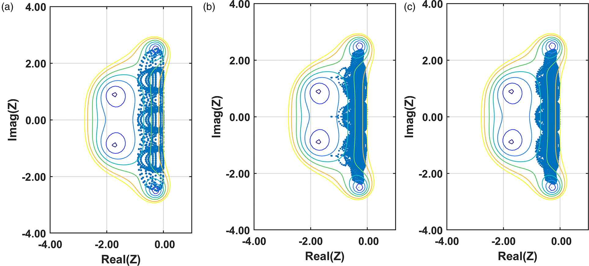
The stability analysis results are presented in Figure 6. Figure 6a and b present the eigenvalue spectra of the transform matrix obtained from the uniform flow field and the nozzle flow field with the fourth combination of boundary conditions, respectively. At the inlet boundary, the static pressure is extrapolated, denoted as inlet1. When using the steady solution of the nozzle as the baseline, the eigenvalues move along the real axis towards the negative direction, approaching the stability boundary. The resulting stability is reduced. To mitigate the instability caused by the nozzle flow field, the Riemann invariant extrapolation is applied at the inlet, denoted as inlet2. Figure 6c shows the eigenvalue spectrum obtained from inlet2 boundary condition. It can be seen that some leftmost eigenvalues in Figure 6b disappear in Figure 6c, indicating that the Riemann invariant extrapolation improves the solution stability and damping property.
Figure 6.
The eigenvalue spectra of the transform matrix for different baseline flow fields and inlet boundary conditions. ( k ( 4 ) = 0.021 , σ = 3 )
For an unsteady flow analysis using the harmonic balance method, the solution stability is compromised by the time spectral source term. In the von Neumann analysis or the matrix analysis, the time spectral source term introduces a pure imaginary value into the Fourier symbol or the eigenvalues, resulting in a shift of them along the imaginary axis in the complex plane, as illustrated in Figure 7. The extent of this shift is associated with a dimensionless parameter, the maximum grid-reduced frequency, defined as
Figure 7.
The locus of the Fourier symbol and the eigenvalue spectrum of the transform matrix ( ω x = 1 , σ = 1.4 )
where
To verify the results obtained from the stability analysis, the flow field within the nozzle configuration was analyzed by our in-house solver. A sinusoidal static pressure is prescribed at the outlet. The periodic unsteady flow induced by the pressure perturbation is solved through the harmonic balance method with a single harmonic. The maximum grid-reduced frequency varies from 0 to 8 though altering the frequency of the unsteadiness. Two subsonic inlet boundary conditions, named inlet1 and inlet2, are implemented in the solver. inlet1 represents the extrapolation of static pressure and inlet2 represents the extrapolation of the Riemann invariant. When the maximum grid-reduced frequency is set to
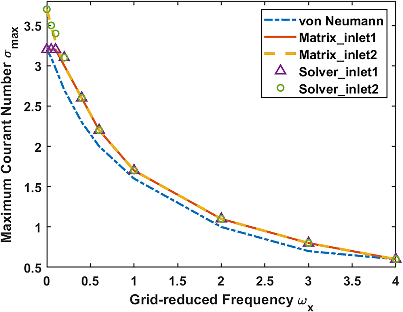
As the maximum grid-reduced frequency increases, the maximum allowable Courant number decreases quickly. Moreover, The maximum allowable Courant numbers with the two different inlet boundary conditions, obtained by numerical experiments, are in good agreement with the matrix analysis results. When it comes to the von Neumann analysis with the assumption of periodic boundary conditions, the predicted maximum allowable Courant numbers are slightly smaller than those obtained by the matrix method at some maximum grid-reduced frequencies, although they are still in good agreement with the results from the numerical experiments.
The stability of the LU-SGS method with the block Jacobi method
The explicit scheme encounters stability issues when it is used to solve the harmonic balance equation, due to the stiffness of the time spectral source term, especially with a large grid-reduced frequency. To stabilize a harmonic balance solution, two implicit methods are presented. The LU-SGS method was first proposed as an implicit preconditioning of the Runge-Kutta method to improve the stability of a steady solution. It can be applied directly to solve the harmonic balance equations without incorporating the Jacobian matrix of the time spectral source term on the left-hand side. It can also be combined with the Block Jacobi method to integrate the time spectral source term implicitly (Wang and Huang, 2017). To assess the stability of these two implicit methods, a von Neumann analysis is conducted.
In the stability analysis, a uniform flow with a Mach number of
Figure 9.
The Fourier symbol loci for different maximum grid-reduced frequencies ( σ = 1000 , ε = 0.6 ) ω x = 0 ω x = 0.2 ω x = 0.5 ω x = 0.5
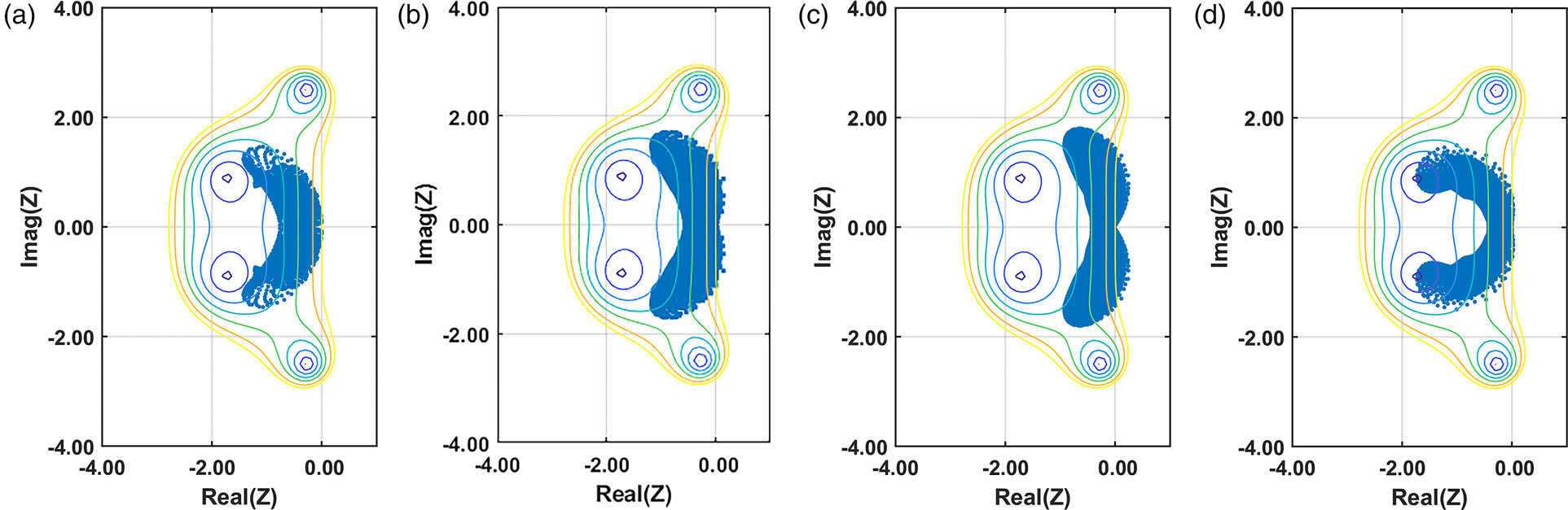
For the harmonic balance equation system, the locus of the Fourier symbol of the LU-SGS method is influenced by the time spectral source term. When the maximum grid-reduced frequency is increased from 0 to 0.2, the locus near the imaginary axis moves to the right side, as shown in Figure 9b. When the maximum grid-reduced frequency reaches 0.5, the locus extends beyond the stability boundary of the classic four-stage Runge-Kutta scheme, shown in Figure 9c. Consequently, the magnitude of the amplification factor is larger than unity and the scheme becomes unstable. To stabilize the solution, the block Jacobi method is used with the LU-SGS method to deal with the time spectral source term implicitly. In Figure 9d, the Fourier symbol locus is restricted within the stability domain when the maximum grid-reduced frequency is set to
To further examine the stabilization effect of the LU-SGS/BJ method, we consider a sufficiently large maximum grid-reduced frequency in the stability analysis. In Figure 10a, the Fourier symbol locus of the LU-SGS method lies outside the stability domain when the maximum grid-reduced frequency
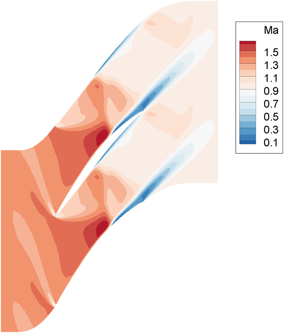
To verify the stability results obtained through the von Neumann method, the NASA rotor 37 is employed as a more realistic test case. The computational domain consists of one blade passage. The domain is discretized using an H mesh with 57 grid points in the radial direction, 49 grid points in the circumferential direction, and 137 grid points in the streamwise direction, among which 72 grid points are on the blade surface (one side only). At the inlet, the total pressure
Figure 11.
The Mach number contours of the NASA rotor 37 at 50% blade span from the solution of the 3-D steady RANS equation.
Then an unsteady analysis is conducted by varying the static pressure periodically in time at the outlet. The harmonic balance method is used to analyze the unsteady flow with a single harmonic. The maximum grid-reduced frequency varies from
Figure 12.
The convergence histories of Res(ρ) solved using the LU-SGS method and the LU-SGS/BJ method ( ε = 0.6 )
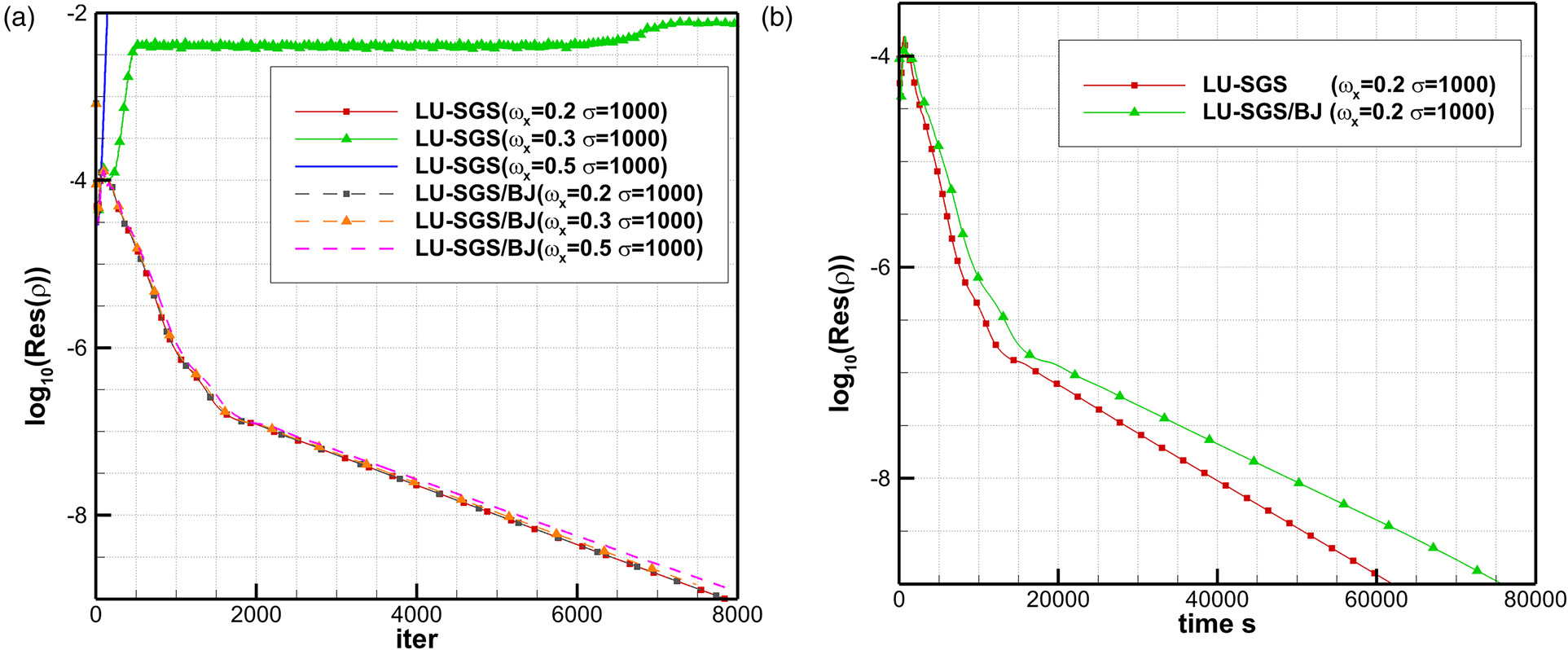
Furthermore, the numerical experiments of NASA rotor 37 with the maximum grid-reduced frequency of 2 are conducted by increasing the unsteady frequency. The convergence historyies of the density equation residual for different implicit methods are shown in Figure 13a. It can be observed that the solution solved with the LU-SGS method can only converge with a very small Courant number, approximately equal to 1. However, with the LU-SGS/BJ method, the maximum Courant number can reach up to
Figure 13.
The convergence histories of Res(ρ) for the LU-SGS method and the LU-SGS/BJ method ( ε = 0.6 )
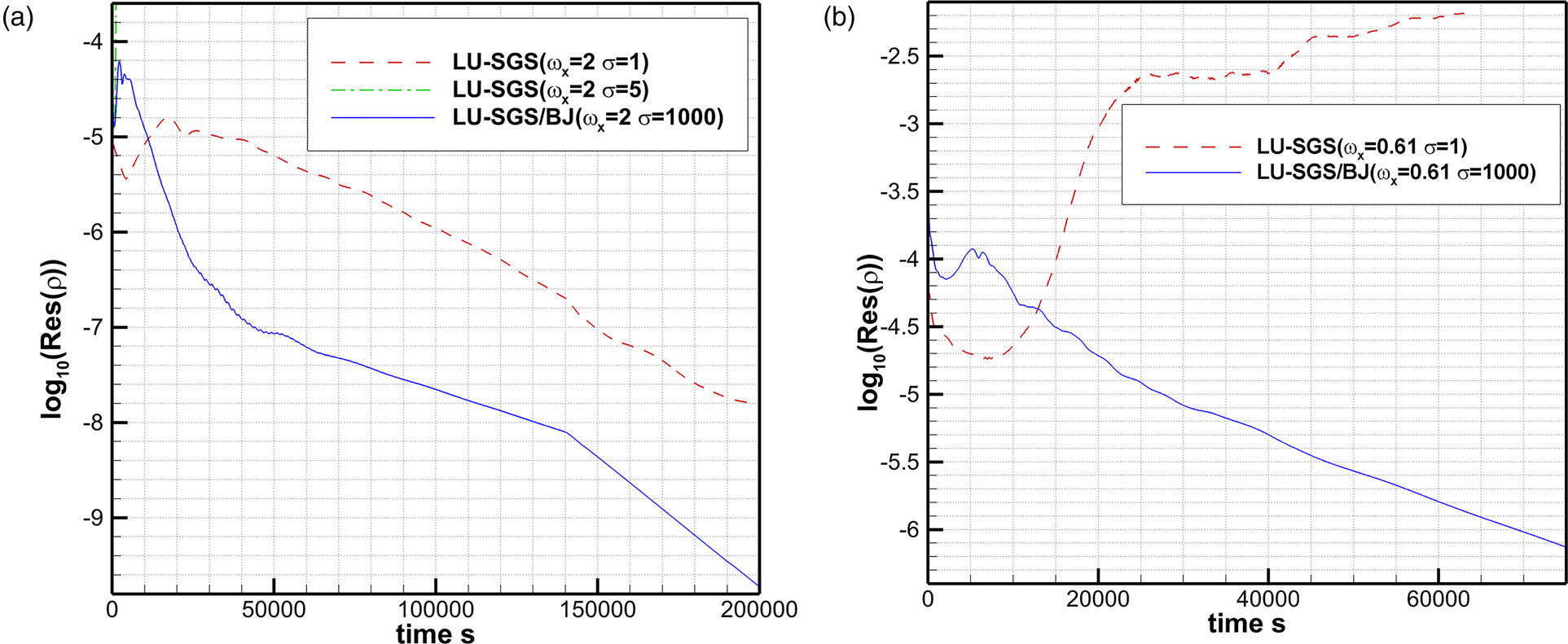
The LU-SGS/BJ method demonstrates a significant reduction in total CPU time, requiring approximately
Conclusion
In this work, we have investigated the stability of the solution methods for steady and harmonic balance equations by using the von Neumann method and the matrix method. These two approaches show identical stability analysis results of the steady Euler equations with periodic boundary conditions. While the eigenvalue spectrum of the system transform matrix changes dramatically with other boundary conditions such as inlet, outlet, and slip wall boundary conditions. Furthermore, the matrix method reveals that stability can be improved by using the Riemann invariant extrapolation at an inlet. For the harmonic balance equations, our stability analysis also demonstrates that the time spectral source term leads to a shift along the imaginary axis in the Fourier symbol locus and the eigenvalue spectrum. Consequently, a smaller allowable Courant number is required to ensure a stable solution with an increasing maximum grid-reduced frequency.
To mitigate the impaired solution stability caused by the time spectral source term, the LU-SGS method and the LU-SGS/BJ method are considered in our analysis. In both the von Neumann stability analysis and numerical experiments, the LU-SGS/BJ method can effectively address the stiffness associated with the time spectral source term, while the LU-SGS method fails with a large maximum grid-reduced frequency. Nevertheless, the implementation of the block Jacobi method incurs additional computational costs. To balance stability and computational efficiency, it is recommended that the LU-SGS method alone be used for cases with a maximum grid-reduced frequency