
Introduction
Hydrogen, as a kind of clean energy, plays an important role in the power industry, especially when it is produced from renewable energy sources (solar and wind) or nuclear energy (Chiesa et al., 2005).
While hydrogen energy technology is becoming more mature, power generation systems based on hydrogen could be an important alternative to conventional power systems based on the combustion of fossil fuels (Milewski, 2015). Mixed hydrogen and pure hydrogen combustion in gas turbines is an important technological path to achieve carbon neutrality.
In response to the energy crisis of the last century, Westinghouse has worked to develop a hydrogen-fueled combustion turbine system designed to meet the goals set by the Japanese WET-NET Program (Bannister et al., 1999; Yang, 2006). Then, several proposed steam turbine thermodynamic cycle configurations, such as GRAZ (Desideri et al., 2001), TOSHIBA (Moritsuka and Koda, 1999), WESTINGHOUSE (Bannister et al., 1998), and MNRC (Miller et al., 2000) are presented. The efficiency of these cycles can achieve as high as 66.4%. The heating value of hydrogen is much higher than traditional fossil fuels. In addition, considering the fact that Hydrogen-Fueled Combustion Turbine Cycle almost eliminates CO2 and NOx emissions, this solution could be viewed as an interesting alternative for future development compared to conventional power technologies.
It is sure that the turbine efficiency and cooling flow requirements have a considerable effect on the cycle efficiency (Scaccabarozzi et al., 2019). Therefore, in order to assess the performance of novel cycles, it is necessary to perform a preliminary evaluation of the turbine efficiency and cooling flow requirements based on a few (or even without) experimental data. Many models have been developed to estimate the cooling flow requirements and turbine efficiency for conventional gas turbines (working fluid is air). These models only depend on the geometric parameters of turbines and the behavior of the working fluid. Halls (1967), Holland and Thake, proposed the first semi-empirical cooling model. El-Masri (1986) proposed a cooling model, which treated the turbine as an expender whose walls continuously extract work. Consonni (1992) proposed the analytical model which considered the blade as a heat exchanger and calculated the distribution of the temperature of the coolant and the cooling efficiency. In the CO2 cycle (working fluid is CO2), Jordal et al. (2004) used El-Masri’s cooling model to evaluate the performance of the semi-closed O2/CO2 cycle with CO2 capture. Fiaschi et al. (2009) used the semi-empirical cooling model to evaluate the performance of an oxy-fuel combustion CO2 power cycle. Scaccabarozzi et al. (2019) applied the analytical model to assess the performance of the cooled supercritical CO2 turbine for the conceptual design.
In this paper, a methodology is proposed for the preliminary evaluation of the turbine efficiency and cooling flow requirements of a novel cycle based on the Hydrogen-Fueled Combustion Turbine Cycle. The thermodynamic analysis and optimization of the cycle are reported in the reference (Yu et al., 2023). Firstly, the novel cycle is shown in section 2. In section 3, the thermodynamic model used in this study is derived. Then, the results are discussed in section 4. At last, the conclusions are summarized in section 5.
The novel H2/O2 cycle
In this research, a novel H2/O2 cycle is operated with pure hydrogen which is fired with pure oxygen (Yu et al., 2023). The stoichiometric oxygen-hydrogen ratio has been taken in this analysis, so the flue gas of this novel H2/O2 cycle is pure steam.
It is a diffluent flow recompression novel H2/O2 combined cycle which consists of the top cycle (red lines) and bottom cycle (blue lines). The top cycle is carried out by gas turbines and the bottom cycle is carried out by ultra-supercritical unit. Figure 1 presents a principal flow scheme of the novel cycle. The top cycle includes components 1–6. Hydrogen and oxygen enter the combustion chamber (component 1, CC) from outside. The working fluid exits the combustion chamber with a temperature of 1,500 °C and a pressure of around 3,800 kPa and then it is expanded to around 102 kPa (component 2, HTT). Cooling is done with a further recycled H2O stream. The energy of the turbine exhaust gas is used to heat the recycle stream in the recuperator (component 3, HRSG). After the recuperator, the cycle fluid is divided into two parts (red line and blue line). Part of the working fluid is compressed by the low-pressure compressor (component 4, C1). The working fluid is cooled by other steam streams in the intercooler (component 5). Finally, the working fluid is compressed again by the high-pressure compressor (component 6, C2).
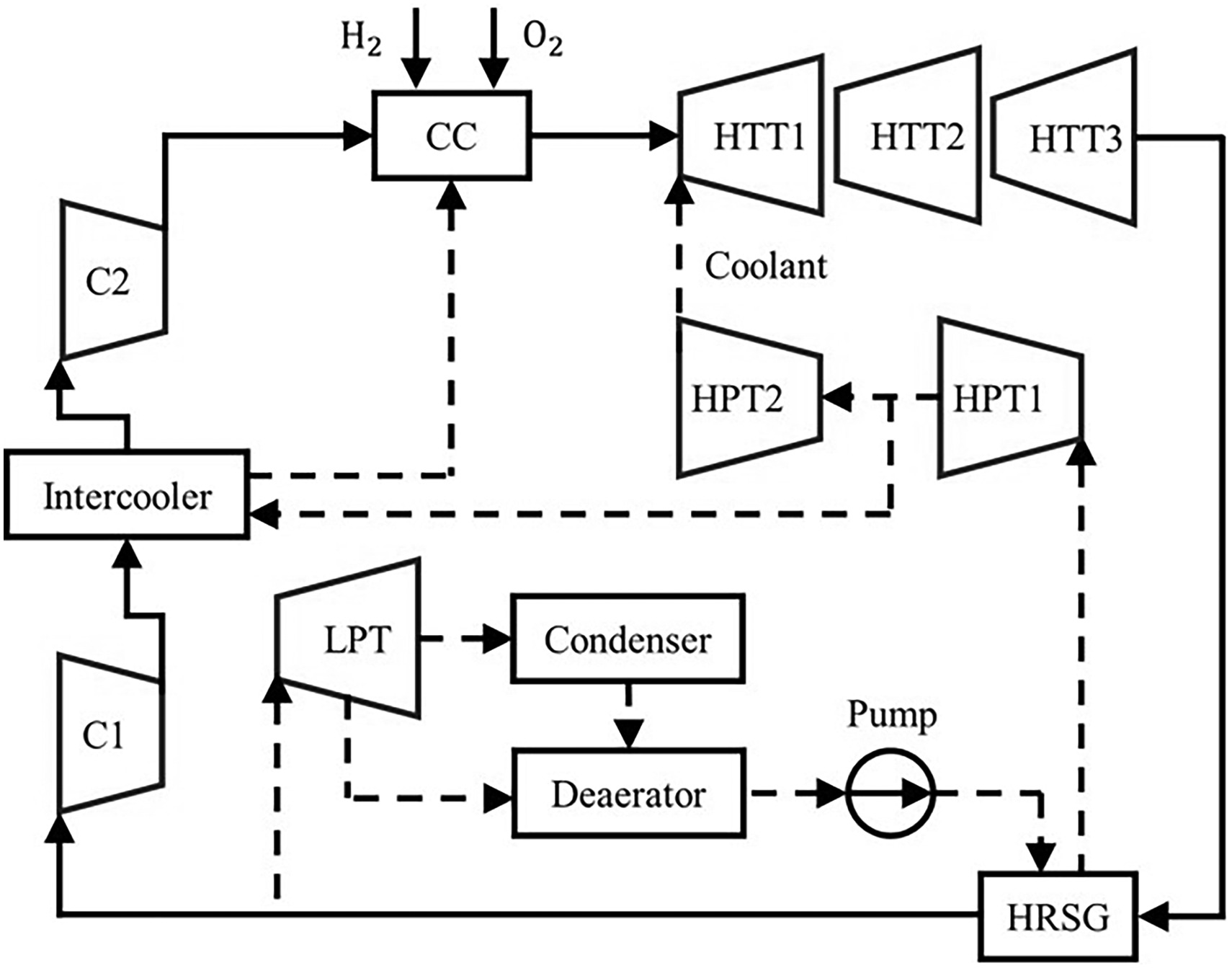
The other part of working fluid separated (blue line) enters the bottom cycle and is expanded in the low-pressure steam turbine (component 7, LPT). Part of steam condenses into water during the expansion and enters the deaerator (component 10). The rest part of steam enters condenser 8 and pump 9, then mixes with the former in the deaerator (component 10). All of the condensates are pumped into the recuperator by the feed pump 11. The condensate is heated by the turbine exhaust gas in the recuperator (component 3, HRSG) and exits as high-pressure steam. This recycled steam is expanded in a high-pressure steam turbine (component 12, HPT1). Part of the exhaust steam enters the intercooler to cool the steam in the top cycle, and the other part of steam is expanded in a medium-pressure steam turbine (component 13, HPT2). The flue steam is used to cool the gas turbine.
This is an advanced form of the thermal cycle for future power generation systems. It can not only achieve the requirement of high efficiency (>70%), but also minimize carbon emissions, or even zero emissions. The working fluid in the top cycle and bottom cycle are both steam so they can mix while the working medium is still pure steam, which is more flexible than the conventional gas-steam combined cycle.
Methodology
The cooling model
In order to predict the cooling flow requirements and their effect on the turbine efficiency, a cooling model is presented. This model is a modification of the model proposed in the reference (Masci and Sciubba, 2018), henceforth referred to as the analytical model.
The blade channel is divided into many elementary layers along the span in the analytical model, as shown in Figure 2. The corresponding blade area of this elementary layer is,
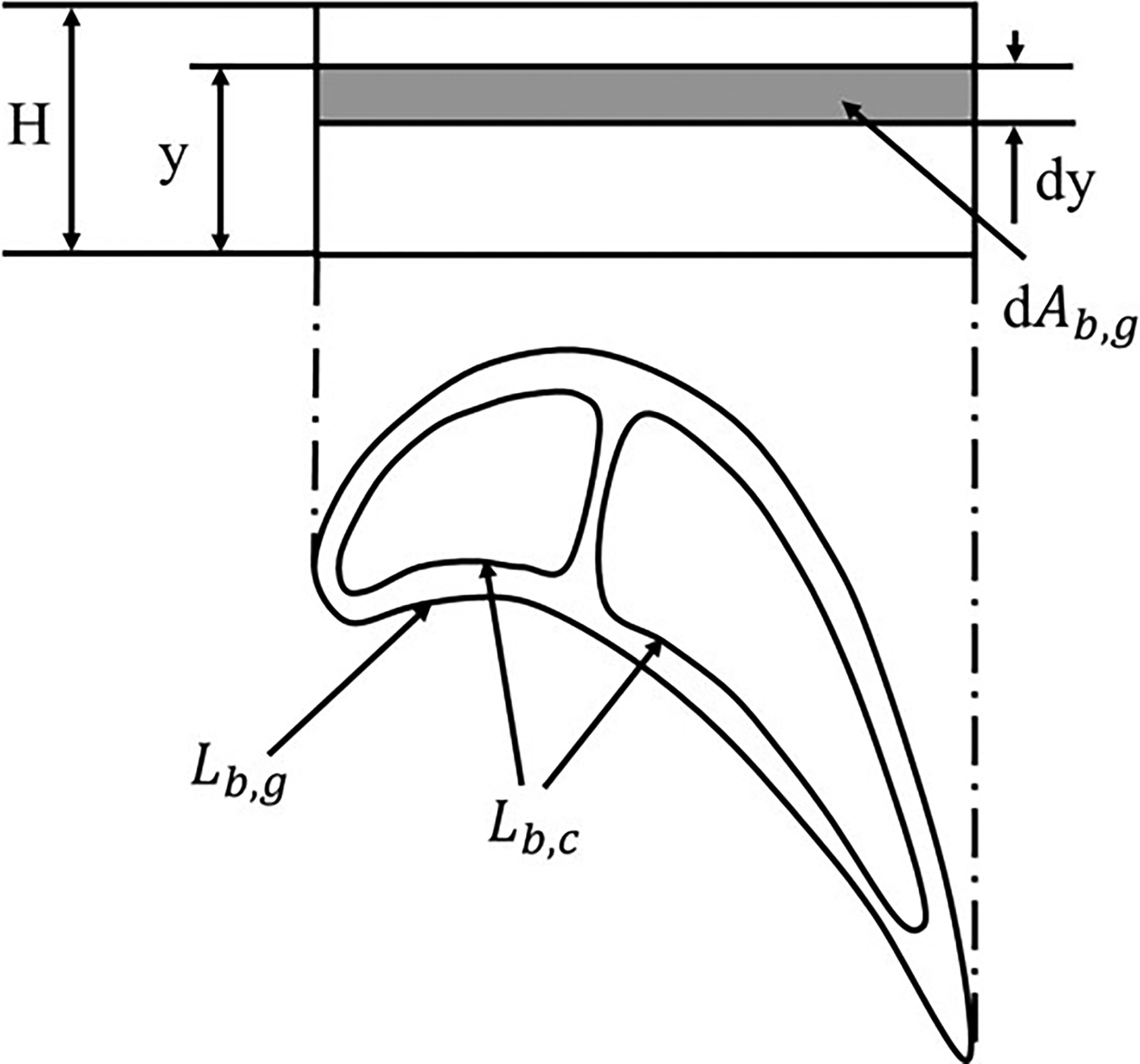
where,

where,
In each elementary layer, it is assumed that
The heat transfer process is steady.
The inlet gas temperature
The heat transfer coefficient keeps constant along both the span and chord.
The conduction along the span is neglected.
The centrifugal effect of rotation on coolant is not considered.
Then the sum of three Equations 3–5 yields
Let
The overall heat transfer coefficient k is used to simplify the notation.
where,
In the internal cooling channel, the temperature of coolant increases due to heat transfer, which is governed by the conservation of energy,
hence
The integration of this equation is then carried out along the span with the gas side perimeter
Hence
where,
which is limited by metallurgical considerations.
The heat transfer coefficient presented in Equation 12 can be calculated with Stanton number, namely,
In the present paper, the external Stanton number is obtained from an empirical equation, as previously employed by Bergman et al. (2011),
The cooling side heat transfer coefficient required by the analytical model can be determined by another empirical Equation 15 proposed by Colburn (Torbidoni and Horlock, 2005),
where,
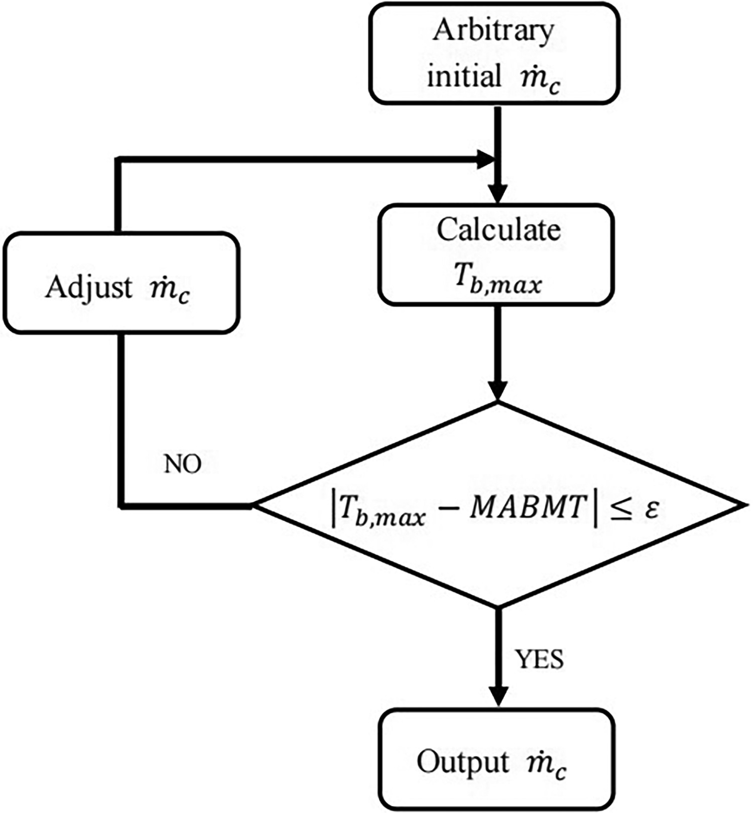
An iterative process is presented in this research aimed to predict the coolant consumption with a given maximum allowable blade material temperature (MABMT) shown in Figure 4.
Select any value as input for the initial coolant mass flow rate.
Calculate the maximum blade temperature.
If the calculated result is higher than the maximum allowable blade material temperatures, the coolant mass flow rate will be increased; otherwise, the coolant mass flow rate will be reduced.
Iterate until the difference between the maximum blade temperature and the maximum allowable blade material temperatures reaches the given precision.
Output the final coolant mass flow rate.
Then,
The film cooling effectiveness is obtained by using empirical Equation 17 proposed by Goldstein (1971).
where,
Cooled expansion
In the present paper, it is assumed that the work is extracted from the expanding gas continuously rather than discretely, therefore, the turbine is considered as an expander. The evaluation of turbine loss and turbine work output can be obtained by following processes.
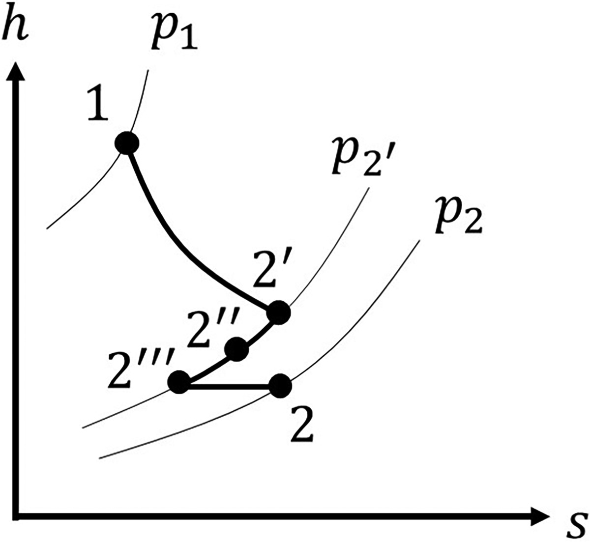
The expansion in the gas turbine is assumed to be a polytropic expansion process in each row (Figure 5, 1–2′), so the temperature at any point of expansion can be obtained by using:
The losses occurring due to internal cooling leads to an isobaric temperature drop during the expansion in a particular row (Figure 5,
The losses associated with the mixing of hot steam and coolant result in another isobaric temperature drop which can be calculated by solving the enthalpy balance equation (Figure 5,
The mixing pressure loss which is considered at the exit of the cooled row makes the state move from point
The work done by one row can be calculated by the following equation. The turbine work is the sum of work done by all rows cooled and uncooled.
The efficiency of turbine is defined as the ratio of the actual turbine specific work to the corresponding isentropic work.
The properties of steam
The equation of state for steam can be obtained from IAPWS-IF97 which is adopted by the International Association for the Properties of Water and Steam (IAPWS) (Wagner et al., 2000). The dynamic viscosity of steam is calculated by using Sutherland’s law (White and Majdalani, 2006):
where,The specific heat of steam is known to be a function of temperature and pressure. However, in the present work specific heat of steam is assumed to be a function of temperature only, represented in the form of polynomials adopted from IAPWS-IF97 as follows:
Some main coefficients of the polynomial are shown in Table 1.Results and discussion
The cooling flow requirements of a typical gas turbine
Compared with a conventional gas turbine, the cooling flow rate of a typical high-temperature turbine is estimated with steam as both working fluid and coolant. In this paper, GE-E3 high-pressure turbine blade is selected and the detailed information can be found in the literature (Timko, 1984). This blade has 2 internal cooling passages where internal cooling can be implemented by flowing the coolant. Additionally, to prevent the hot main annulus gas of the turbine from overheating and damaging the blade, film cooling is applied to reduce the heat load.
Coolant consumption against gas temperature for steam and air as the working fluid is shown in Figure 6. The different solid line represents different coolant inlet temperature for air (500 K–900 K), similarly, the different dashed line represents different coolant inlet temperature for steam (500 K–900 K). The coolant consumption with air or steam as coolant increases with an increase in gas temperature almost linearly. For GE-E3, the inlet temperature is 2,012 K and coolant inlet temperature is 883 K at the design point. Hence, the corresponding coolant consumption is 6.31% which is close to the actual value of 6.3%. Therefore, the analytical model has been verified to be valid.
Figure 6.
Effect of gas temperature and coolant inlet temperature on coolant consumption for steam and air as cooling medium.

At a coolant inlet temperature of 500 K, the coolant consumption with steam as cooling medium is 24.73%, 22.89%, 21.19%, 19.54%, 17.89% and 16.25% less in comparison to the coolant consumption with air as cooling medium for gas temperature is 1,500 K, 1,600 K, 1,700 K, 1,800 K, 1,900 K and 2,000 K, respectively. It is reasonable that the specific heat capacity of steam is larger than that of air. However, at a coolant inlet temperature of 600 K, 700 K, 800 K and 900 K, the amount of cooling flow rate is more by applying cooling steam. The difference between performance of air cooling and steam cooling can be defined as:
Table 2.
The difference between air cooling and steam cooling (Δ).
The performance of novel H2/O2 cycle turbine
The overall structure of turbines includes three cylinders which consist of high-pressure gas turbine, medium-pressure gas turbine and low-pressure gas turbine denoted by HTT1, HTT2 and HTT3 respectively. HTT1 and HTT2 are driven by high-pressure and low-pressure axial flow compressors respectively and HTT3 is a power turbine. Figure 7 shows the cross-sectional view of the turbines. Detailed information on the three turbines is reported in Table 3. The coolant inlet temperature is low so that the coolant consumption can be reduced with steam cooling.

Table 3.
Turbine analysis data.
| Value | Turbine | |||
|---|---|---|---|---|
| HTT1 | HTT2 | HTT3 | ||
| Parameter | Pressure ratio | 1.31 | 1.76 | 16.24 |
| Coolant inlet temperature (K) | 567.52 | 531.85 | 476.48 | |
| Number of stages | 1 | 2 | 5 | |
| Polytropic efficiency | 0.91 | 0.91 | 0.91 | |
The H2/O2 cycle studied in this paper is the optimized case presented in the reference (Yu et al., 2023). The resulting turbine operating conditions are:
The calculation is carried out for the uncooled case first and then for the cooled case to reveal the impact of cooling system on the performance and expansion. Both cases use the same inlet conditions.For the cooled case, two kinds of maximum allowable blade material temperature distributions are applied. One is that the maximum allowable temperature remains unchanged at 1,250 K for all rows. However, materials with high melting points cost a lot, so in practice, it decreases along the expansion. Therefore, the other is that the maximum allowable temperature takes the value of 1,250 K, 1,200 K and 1,000 K for HTT1, HTT2 and HTT3 respectively.
The results related to the novel H2/O2 cycle turbine are represented in Table 4. It shows that all stages in HTT1 and HTT2 are cooled but in HTT3 only part of stages are cooled because the gas temperature is less than the allowable blade material temperature. The coolant consumption of any cooled row is less than 2%. The coolant mass flow rate and film cooling effectiveness decrease during the expansion in an individual turbine.
Table 4.
Film cooling effectiveness and coolant consumption of each row.
Note that the film cooling effectiveness values obtained here are lower than the ones reported in the literature for a conventional modern gas turbine, where it can arrive 0.3 (Uysal, 2020). The reason maybe is that the coolant consumption is less when the working fluid and coolant are both steam according to the previous section and less coolant is required for film cooling than conventional gas turbines, so the film cooling effectiveness is less.
The comparison of performances is reported in Tables 5 and 6. For the case with different maximum allowable blade material temperatures, the isentropic efficiency with consideration of the cooling effect of three turbines is 1.29%, 1.72% and 3.39% less than those without consideration of the cooling effect, respectively. The losses caused by cooling system increase with the increase of coolant consumption.
Table 5.
The isentropic efficiency for the uncooled and the cooled cases.
| Isentropic efficiency | Turbine | ||
|---|---|---|---|
| HTT1 | HTT2 | HTT3 | |
| Uncooled | 91.20% | 91.64% | 93.46% |
| Cooled (different maximum allowable temperature) | 89.91% | 89.92% | 90.07% |
| Cooled (uniform maximum allowable temperature) | 89.91% | 90.17% | 92.86% |
Table 6.
The actual specific work for the uncooled and the cooled cases.
The performance of HTT1 and HTT2 are almost the same for the cases with different and uniform maximum allowable blade material temperatures. For the last turbine with uniform maximum allowable blade material temperature, since 6 rows are not cooled, the isentropic efficiency and specific work are closer to the uncooled case.
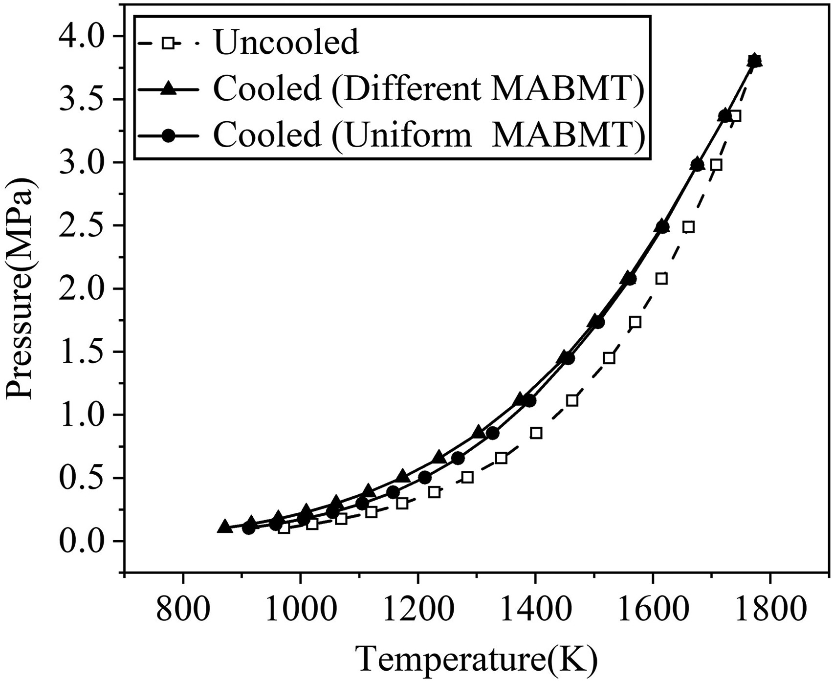
Steam pressure against temperature is shown in Figure 8. The two p-T curves on the left (solid line) represent the cooled turbine while the p-T curve on the right (dashed line) represents the uncooled turbine. It is illustrated that the temperature of the main stream of cooled turbine with uniform maximum allowable blade material temperature is a little higher than that of cooled turbine with different maximum allowable blade material temperatures, and they are both lower than that of uncooled case.
Conclusions
In this paper, the analytical model is used to compare the cooling performance with the different cooling mediums (air and steam). A methodology for the preliminary performance estimation without experimental data of the novel H2/O2 cycle turbine is presented. All stages in HTT1 and HTT2 are cooled but in HTT3 only part of stages is cooled to protect the blade from hot gas.
Main conclusions are summarized as follows:
The result obtained by applying analytical model on GE-E3 high-pressure turbine agrees well with the design data, which demonstrates that the model is valid.
The coolant consumption with steam as cooling medium is less in comparison to the coolant consumption with air as cooling medium because the specific heat capacity of steam is larger than that of air at low coolant inlet temperature. More coolants are required by applying steam cooling at high coolant inlet temperature. The difference between performance of air cooling and steam cooling decreases with increase in gas temperature and first decreases and then increases with increase in coolant inlet temperature.
The amount of coolant used for film cooling with steam as cooling medium is less than that with air as cooling medium and the film cooling effectiveness values obtained here are lower than the ones reported in the literature for a conventional gas turbine. The penalty due to applying cooling system is significant. Like specific work, the isentropic efficiency with consideration of the cooling effect of HTT1, HTT2 and HTT3 is 1.29%, 1.72% and 3.39% less than those without consideration of the cooling effect, respectively.
Nomenclature
Latin symbols
area
specific heat at constant pressure
parameter that considers increased surface of cooling channels due to turbulators
blade height
specific enthalpy
overall heat transfer coefficient
perimeter
blowing rate
mass flow rate
Prandtl number
pressure
heat flux
Reynolds number
Reynolds number based on diameter of film hole
Stanton number
diameter of film hole
temperature
velocity
molecular weight
specific work
distance from point of injection
radial [span-wise] coordinate