Geometry and mesh of the NACA0009 hydrofoil

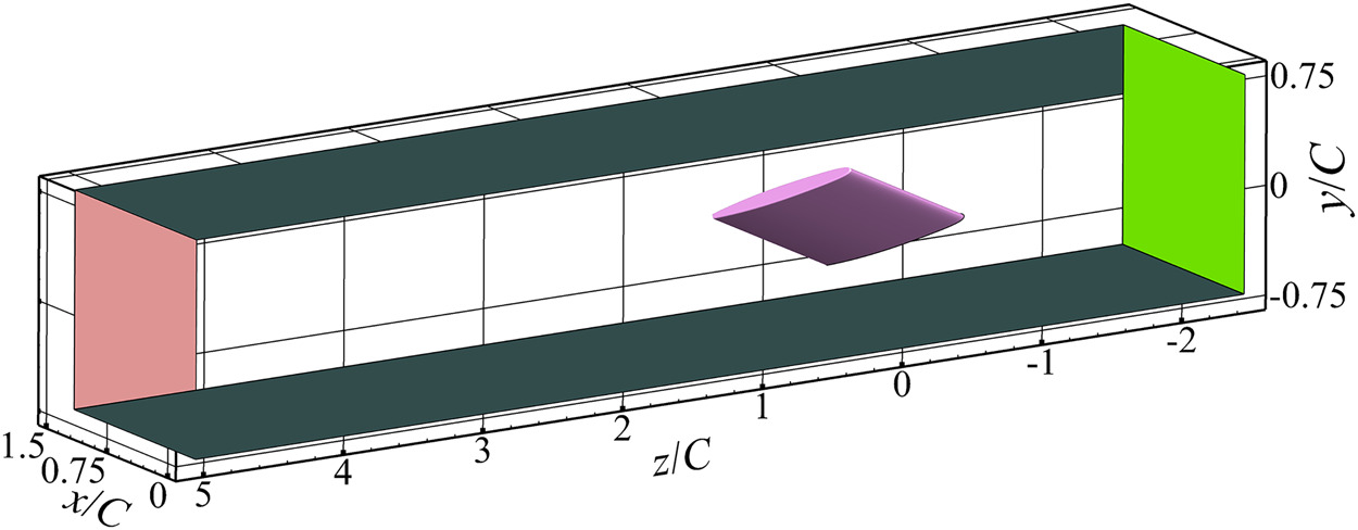
According to the experiments (Dreyer et al., 2014; Dreyer, 2015), the geometry and computational domain of the NACA0009 hydrofoil are shown in Figure 1. The incidence angle is 10° with a chord length (C) of 100 mm. The maximum thickness of the hydrofoil is 9.9 mm, and the thickness distribution is referred to Dreyer et al. (2014). The computational domain has a cross section of 1.5C × 1.5C and a length of 7.5C. The reference length (L) of tunnel cross section is defined as 1.5C. The Cartesian coordinate system origin is located at the center of the hydrofoil root. The boundary conditions in numerical simulations are consist with experiment. The inlet is at 2.5C upstream of the coordinate system origin. Inlet velocity (U) is 10 m/s with a turbulence intensity of 1%, and inlet time-averaged pressure (p∞) is kept to 1 bar. The non-slip boundary condition is applied to walls of the tunnel and hydrofoil. The gap size (h) between the tunnel and hydrofoil tip is varied smoothly between 0C and 0.2C in the experiment. In this study, the cases with non-dimensional gap size (h/C) of 0.1 and 0.01 are studied to have a deeper understanding of the effect of gap size on the evolutions of multi-scale vortical structures and cavities. In this study, the x coordinate is nondimensionalized based on L, that is, the tips of hydrofoil with small and large gap are located at x/L = 14.9/15 and 14/15, respectively.

Figure 1.

Geometry and computational domain of the hydrofoil.

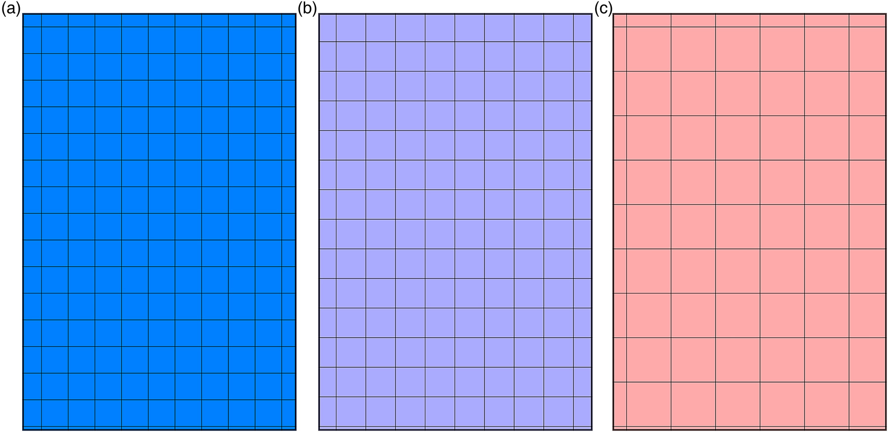
More details of meshes are shown in our previous study (Xie et al., 2023). The fine mesh that contains 11.8 million cells is employed for LES case, and the medium mesh (M1) that contains 7.6 million cells is used for GAS and SAS cases. In this study, the coarse mesh (M2) containing approximately 3.8 million cells is used for GAS cases. Comparation of grid scales in refined region are shown in Figure 2. The minimum grid scales of three meshes are 0.45, 0.5 and 0.75 mm, respectively. The simulation results show that the y+ of the walls is approximately 1, which meets the requirements.

Figure 2.

Comparison of grid scale in refined region. (a) LES (b) GAS M1 (c) GAS M2.

Grid-adaptive simulation

GAS method, a new high-fidelity hybrid RANS-LES method proposed recently (Wang and Liu, 2022), is employed to investigate unsteady cavitating flow around the NACA0009 hydrofoil. The SST model is chosen as the baseline turbulence model of GAS method. The ratio of grid scale to turbulent integral length scale is introduced in GAS to modify the turbulent viscosity in SST model. The modified turbulent viscosity is defined as:

where km and ωm represent the turbulent kinetic energy and specific dissipation rate in SST model, respectively, Df is the factor to rescale the turbulent viscosity:

where lm is the turbulent scale in SST model:

where β∗=0.09, the FGAS and Δ∗ are shielding function and grid scale, respectively:

where Ret is the turbulent Reynolds number, v is the molecular kinematic viscosity, Δvol represents the cube root of the grid volume, and the Δmax is the maximum grid length.

Numerical methods

The commercial software ANSYS Fluent is employed to conduct the numerical simulations. The SIMPLEC scheme is used for pressure-velocity coupling. The second-order scheme is utilized for spatial discretization of pressure equation, and bounded central differencing scheme is applied for momentum equation. The first-order upwind scheme is utilized for the volume fraction equation. The second-order upwind scheme is utilized for turbulent kinetic energy and specific dissipation rate equations. The bounded second-order implicit scheme is applied for transient formulation. Moreover, warped-face gradient correction and high order term relaxation are also used to improve the convergence. The time step is set to 2.5 × 10⁻⁵ s with 20 iterations per time step. The CFL number in flow field is less than 0.5. The statistical quantities of monitoring points in complex flow structures reach statistical convergence, indicating that the simulations meet the requirements.

The mixture model is used to solve the mixture momentum equation. Zwart–Gerber–Belamri (ZGB) cavitation model (Zwart et al., 2004) is utilized to predict the process of phase change in the cavitating flow around a NACA0009 hydrofoil. The interphase mass transfer rate in ZGB model is defined as:

where Fvap=50 and Fcond=0.01 are the empirical coefficients, αnuc=5×10−4 is the volume fraction of nucleation, RB=10−6m is the bubble radius, αv is the vapor volume fraction, ρl=997kg/m3 is the water density and ρv=0.0231kg/m3 is the vapor density. The saturation vapor pressure (pv) is 3170 Pa, which corresponds to an ambient temperature of 25°C. Then the cavitation number and Reynolds number are derived:

To be clear, the methods and computational setup of LES, SAS and GAS M1 cases (Xie et al., 2023) are briefly introduced in this section. In LES, a filtering function is used to divide vortices into large- and small-scale ones. The dynamic Smagorinsky–Lilly model is utilized to model the effects of small-scale vortices, thereby overcoming the limitations associated with constant coefficients. Consequently, the Smagorinsky constant varies in time and space over a fairly wide range. SAS is proposed to resolve the turbulent spectrum in unstable flow by incorporating the von Kármán length scale into the turbulence scale equation. Introducing the von Kármán length-scale imparts an LES-like character in strongly unsteady regions. The primary distinction between SAS and the standard SST model lies in the addition of an extra source term (QSAS) to the transport equation of ω in SAS. Differ from the GAS M2 case, the time steps of LES, SAS, and GAS M1 cases are set to 1 × 10⁻⁵s.

Validation of GAS method

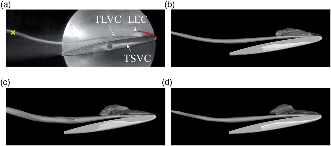
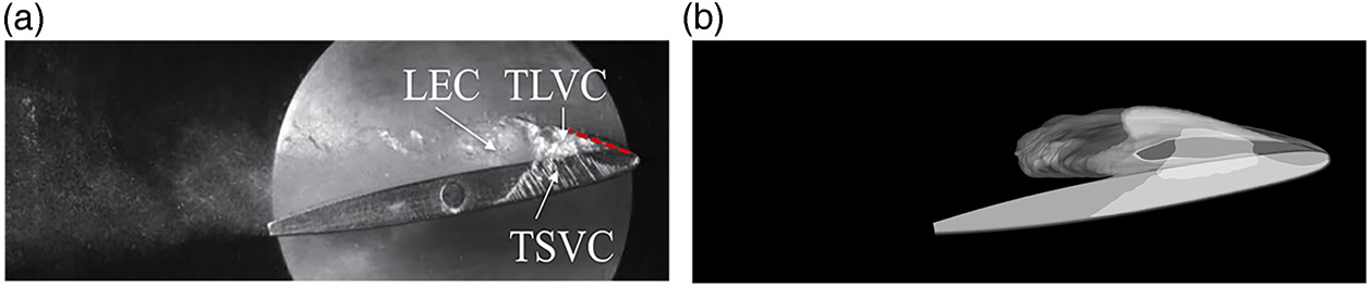
In this section, the GAS method is validated by comparing with the experimental and LES results. Moreover, as shown in Figure 2, grid scale of M2 is significantly larger than M1. Thus, M1 and M2 are used to validate the grid-adaptive ability of the GAS model. Comparisons of predicted and measured time-averaged cavities at h/C = 0.1 are presented in Figure 3. A red dotted line is added to indicate the boundary of the time-averaged LEC. The LEC, TLVC and tip separation vortex cavitation (TSVC) are accurately predicted by GAS on the coarse mesh M2. The scales of these cavities in GAS M2 are agree with the experimental and LES results, indicating that GAS gives a reasonable turbulent viscosity by considering grid scale, and shows a LES-like behaviour.

Figure 3.

Predicted and measured time-averaged cavities (α_v= 0.1), h/C = 0.1 (Dreyer et al., 2014). (a) EXP (b) LES, (c) GAS M1 (d) GAS M2.

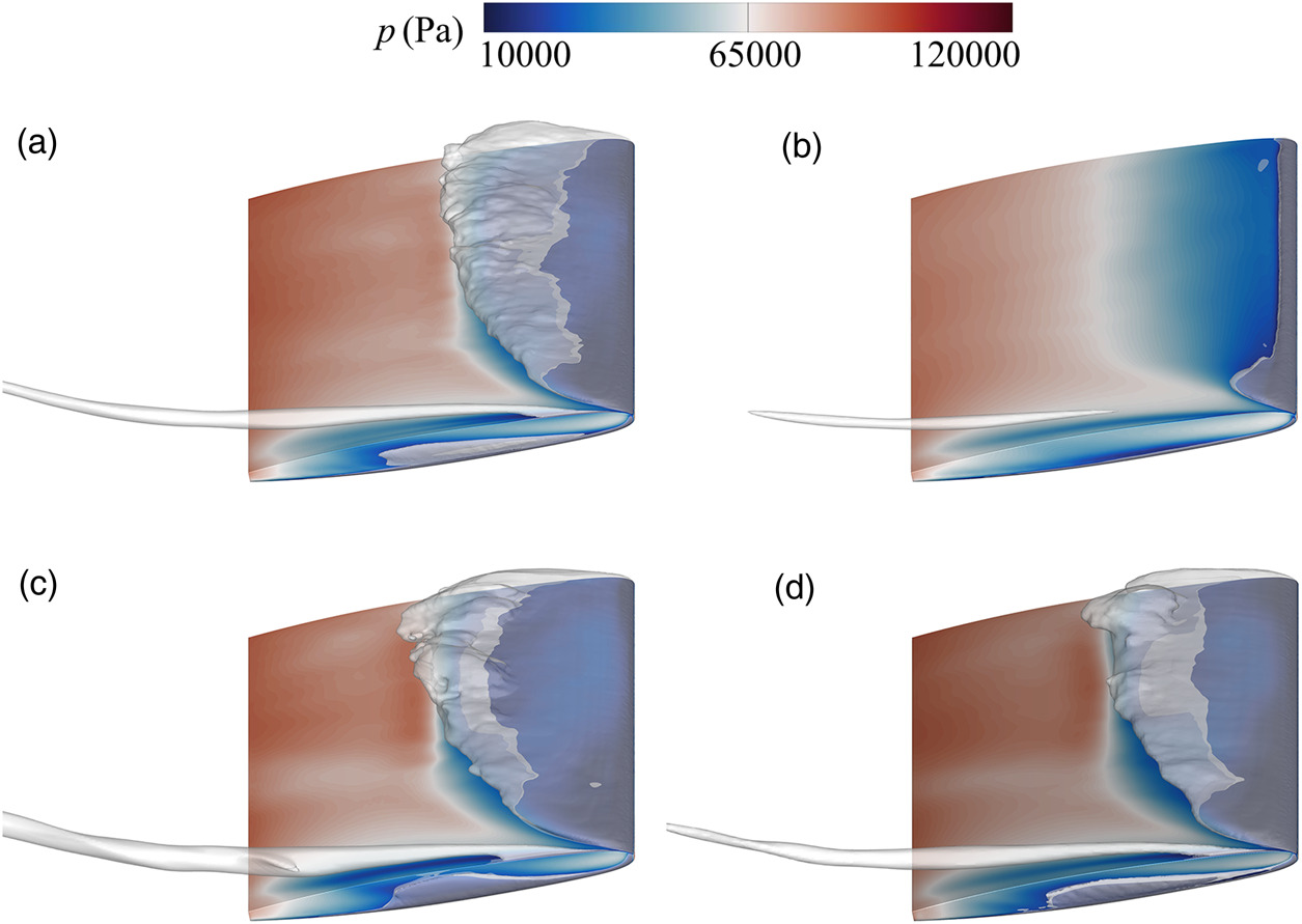
Comparison of time-averaged cavities and blade surface pressure predicted by different methods are also shown in Figure 4. The SAS significantly underestimates the macroscale cavities, especially the LEC. The inception of TLVC is delayed, and the cavity closure occurs more rapidly. Moreover, the SAS does not predict the occurrence of TSVC. The predicted results of GAS M2 are more consist with the LES data than the results predicted by SAS based on M1, showing the ability of GAS to achieve high accuracy with low grid requirement.

Figure 4.

Comparison of time-averaged pressure and cavities (α_v= 0.1) Predicted by different methods. (a) LES, (b) SAS M1, (c) GAS M1, (d) GAS M2.

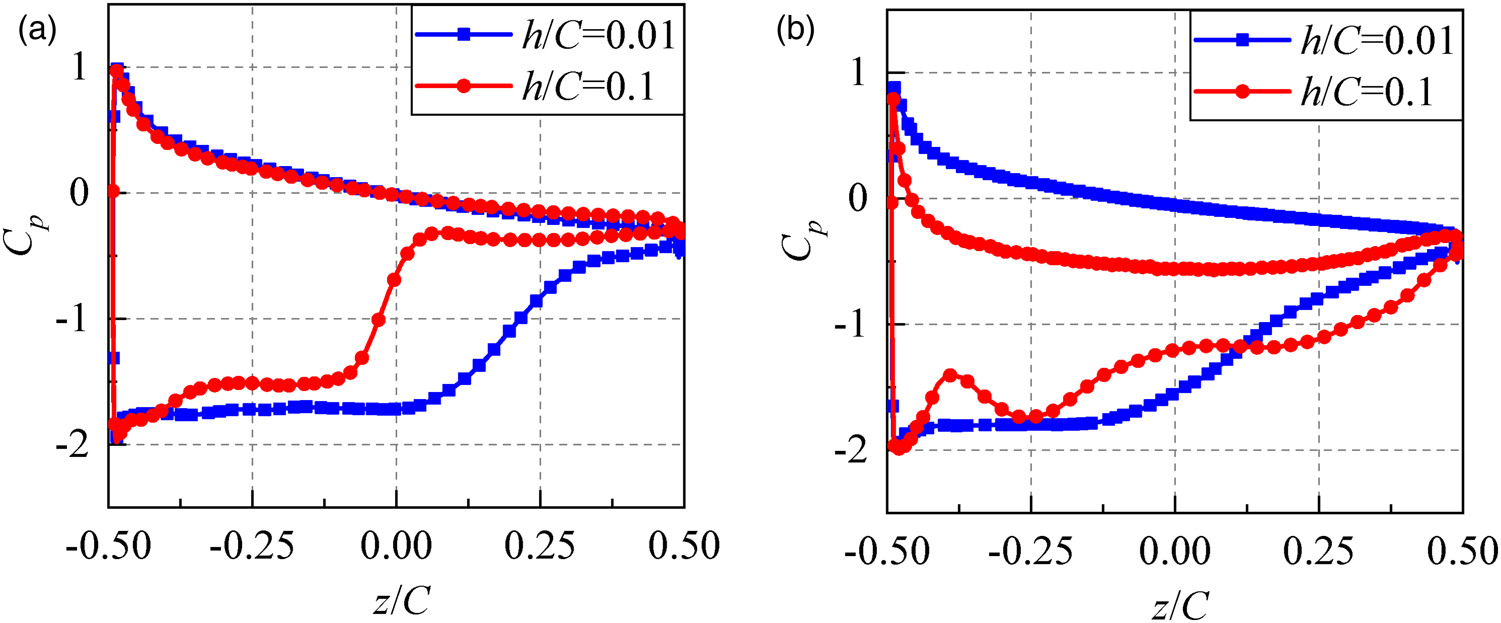
Quantitative comparisons of time-averaged streamwise velocity are shown in Figure 5. The negative streamwise velocity resulted from the re-entrant jet in LEC region is clearly captured by GAS. Both GAS M1 and GAS M2 results have good agreement with the LES data at x/L = 7/15 and x/L = 12/15, indicating that the GAS method has good grid-adaptive ability. Comparison of predicted and measured cavities at h/C = 0.01 are also shown in Figure 6. The key flow structures, such as LEC, TLVC, and TSVC, are clearly captured by GAS, further validating the performance of GAS. In the following sections, the results of the GAS method based on M2 are analysed in detail.

Figure 5.

Comparison of time-averaged streamwise velocity, h/C = 0.1 (Xie et al., 2023). (a) x/L = 7/15, (b) x/L = 12/15.

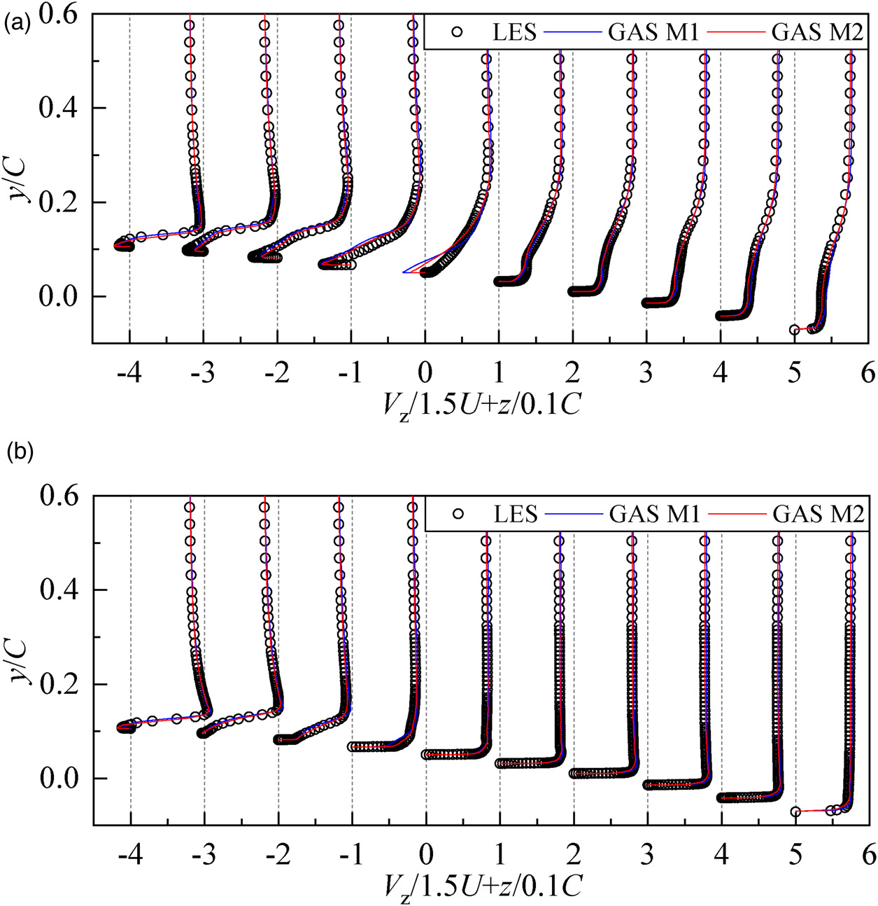
Figure 6.

Predicted and measured cavities (α_v= 0.1), h/C = 0.01 (Dreyer et al., 2014). (a) EXP (b) GAS M2.

Evolution of cavities and vortices

The local trace criterion (LTcri) (Liu and Tang, 2019; Liu et al., 2021) is used to extract multi-scale vortical structures in cavitating flow. In LTcri, Ψ=(∇u)2/2 based on the quadratic velocity gradient tensor is defined, and the value of LTcri is defined as the first invariant of Ψ. The simplified form of the LTcri is:

where Δ represents the discriminant of the velocity gradient tensor (Chong et al., 1990), λr reflects the compressing or stretching rate of the spiral trajectory, λcr is the real part of the complex eigenvalue of the ∇u, representing the radial expansion or contraction, and λci is the imaginary part of the complex eigenvalue of ∇u.

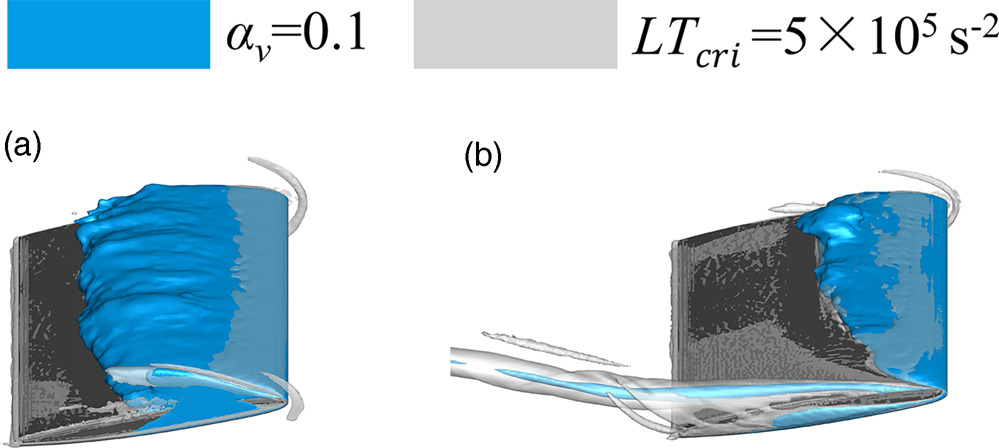
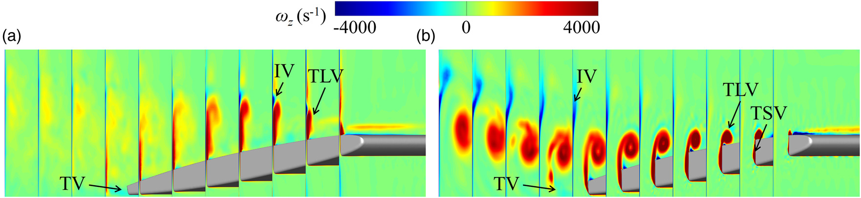
Evolution of cavities and vortical structures within a period (T₁) are demonstrated in Figure 7. At h/C = 0.01, the development of cavities shows periodical growth and collapse. The LEC exhibits a stable sheet cavity attaching to the leading-edge (LE) at 0/4 T₁, and cavity length reaches its maximum at 2/4 T₁. While, the cavity is cut off rapidly, resulting in cloud cavitation shedding at 3/4 T₁. LEC is the most important flow structure in small gap size unsteady cavitating flow. The lengths of the TLVC and TSVC are always smaller than that of LEC. The vortex identification results indicate that there is a significant positive correlation between the TLV breakdown and LEC development. When LEC is cut off at 3/4 T₁, the TLV also becomes instability, with a concentrated vortex breaking into small vortices. It should be noted that some small-scale vortices with higher circulation in cloud cavitation shedding region also form cavities in their core. Moreover, the small gap leads to the formation of horseshoe vortex near the tip, but the cavity does not occur in the vortex core, indicating that the strength of horseshoe vortex is weak. Differ from the small gap condition, the scale of LEC is smaller, while the TLVC and TSVC are longer at h/C = 0.1. The concentrated leakage vortex develops far downstream without breaking. In addition, the horseshoe vortex upstream of the tip also disappears. Time-averaged cavities and vortical structures are depicted in Figure 8. The trajectory of the TLV moves away from the hydrofoil as the gap size decreases. The position of induced vortex is also closely related to the gap size.

Figure 7.

Evolution of cavities and vortical structures. (a) 0/4 T₁, h/C = 0.01, (b) 1/4 T₁, h/C = 0.01, (c) 2/4 T₁, h/C = 0.01, (d) 3/4 T₁, h/C = 0.01, (e) 0/4 T₁, h/C = 0.1, (f) 1/4 T₁, h/C = 0.1, (g) 2/4 T₁, h/C = 0.1, (h) 3/4 T₁, h/C = 0.1.

Figure 8.

Time-averaged Iso-surfaces of cavities and vortical structures. (a) h/C = 0.01, (b) h/C = 0.1.

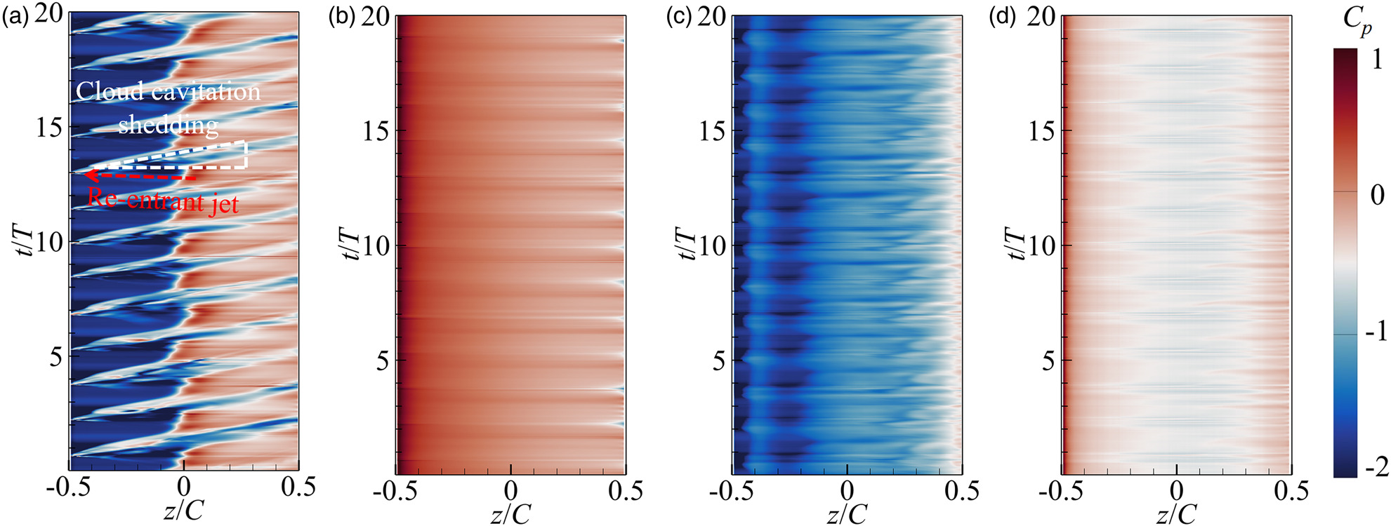
The temporal-spatial distribution of pressure coefficient at h/C = 0.01 is presented in Figure 9 to further investigate the characteristics of LEC. The pressure coefficient is defined as:

Figure 9.

Temporal-spatial distributions of instantaneous pressure coefficient, h/C = 0.01. (a) SS, x/L = 7/15 (b) PS, x/L = 7/15 (c) SS, x/L = 14.7/15 (d) PS, x/L = 14.7/15.

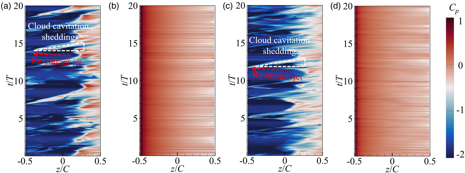
The ordinate represents that the data of twenty reference times (T=C/U) are plotted. According to the relationship between Cp and σ, the Cp lower than −1.94 means that the LEC is attached to the hydrofoil. As shown in Figures 7 and 8, the cavitating flow at h/C = 0.01 shows a quasi-two-dimensional flow; thus, x/L = 7/15 is defined as the mid-span of two gap size cases. As mentioned earlier, the tips of hydrofoil with small and large gaps are located at x/L = 14.9/15 and 14/15, respectively. In this section, a position 2 mm below the hydrofoil tip is defined as near tip, thus the near tip positions of small and large gaps are located at x/L = 14.7/15 and 13.8/15, respectively.

In Figure 9(a), the growth and collapse of the cavity is observed very clearly at mid-span and near tip. At present, it is widely recognized that the large-scale LEC is cut off rapidly by the re-entrant jet with high pressure, resulting in the cloud cavitation shedding. In this study, the re-entrant jet with high pressure is shown by a red dotted line, and the cloud cavitation shedding region is presented by a white dotted line. According to the development of the re-entrant jet, it is believed that jet originates from the closure region of the LEC and flows to the LE, indicating that the cloud cavitation shedding always starts at LE. It should be noted that the velocities of re-entrant jet and cloud cavitation shedding are almost equivalent. Combining with Figure 7, the re-entrant jet is believed to have a strongly interact with the large-scale cavity. This is because the cloud cavitation shedding is induced by the smaller fragmented vortical structures with significant circulation and low pressure in their cores. Consequently, these smaller structures can sustain for a longer time until they collapse near the trailing edge (TE). Another feature observed in Figure 9 is that the flow characteristics at mid-span and near tip are similar, indicating that the flow can be approximated as quasi two-dimensional at h/C = 0.01.

Temporal-spatial distributions of Cp at h/C = 0.1 are shown in Figure 10. A very clear shedding frequency can be observed at mid-span [Figure 10(a)]. In addition to the characteristic frequency and cavity scale, the evolution processes of cloud cavitation shedding and re-entrant jet are basically consistent with that of small gap size. It should be noted that the flow structures near the tip is significant differently from the mid-span, exhibiting strong three-dimensional characteristics. Although the frequency of the low-pressure region on the SS of the hydrofoil tip is consistent with frequency of LEC, the cavity at LE exhibits small-scale attached cavity. There is another low-pressure region at the z/C = −0.25, and the peak value of Cp on the SS of the blade tip appears at the TE, which is also significantly different from the mid-span. The Cp on the PS of the blade tip is also lower, indicating a smaller blade load near tip at large gap size. It is noted that due to the different scales of LEC regions, the frequency of LEC h/C = 0.01 is significantly lower than the frequency at h/C = 0.1.

Figure 10.

Temporal-spatial distributions of instantaneous pressure coefficient, h/C = 0.1. (a) SS, x/L = 7/15 (b) PS, x/L = 7/15 (c) SS, x/L = 13.8/15 (d) PS, x/L = 13.8/15.

Quantitative comparisons of time-averaged Cp on blade surface are shown in Figure 11. The difference of Cp on the PS at mid-span between two gap sizes is negligible. The length of low Cp region is consistent with that of the time-averaged cavities. Moreover, due to the large scale of the cavities at h/C = 0.01, the distance between the cavities and the hydrofoil is smaller. Consequently, the Cp of time-averaged cavities at h/C = 0.01 is still lower than that of the large gap size case. Furthermore, the closure position of the LEC is stable at h/C = 0.1 due to its periodicity, thus the slope of Cp at closure position is large. However, in the case of small gap size, there is no obvious dominant frequency, so the slope of Cp is relatively lower. The difference of Cp near the tip for different gap sizes is more significant. The fluid near the PS of hydrofoil is affected by the unloading of the blade gap, and this effect is positively related to the gap size, so the Cp on the PS is significantly smaller at h/C = 0.1. As shown in Figures 7 and 8, the local minimum Cp at z/C = −0.25 is induced by the TLVC.

Figure 11.

Distribution of time-averaged pressure coefficient. (a) x/L = 7/15 (b) x/L = 14.7/15 at h/C = 0.01, x/L = 13.8/15 at h/C = 0.1.

Effect of gap size on the flow structures evolution

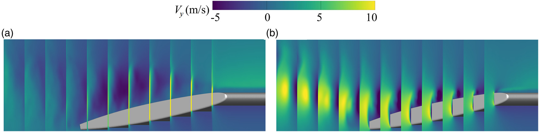
As described above, the gap size has a significant impact on the evolution of cavities and vortical structures. Further research is needed on the interactions of these structures need. Figures 12 and 13 depict the distributions of time-averaged streamwise vorticity and pitchwise velocity. It is found that the TLV at h/C = 0.1 has a larger scale and higher vorticity, while the overall vorticity of TLV at h/C = 0.01 is relatively small. It is noted that the IV at h/C = 0.01 is closer to the upstream. The distribution of radial velocity indicates that the jet velocity is higher near the LE, resulting in local strong TLV and IV near LE. The higher jet velocity also leads to a purely potential effect, namely elevation of the TLV trajectory. Moreover, the tunnel wall also has an effect on nearby TLV, which can be explained by image vortex, further promoting the elevation of the TLV. However, a smaller gap means less leakage flow, affecting the vorticity transport from the tip to the TLV. Thus, the strength of the TLV decreases rapidly under the effect of the boundary layer of the tunnel wall. As shown in Figure 12(b), the TSV begin to merge with TLV at half chord position. The vorticity of TLV further increases due to the supply of tip leakage flow, resulting in the appearance of IV. While the TSV is negligible under the suppression effect of the jet at h/C = 0.01. Furthermore, the streamwise vorticity in the TLVC region at h/C = 0.1 is smaller than that of the vapor-liquid interface, it is on account of the expansion of cavities. Thus, the vorticity of the TLV core is transported to the vapor-liquid interface (Xie et al., 2023).

Figure 12.

Distribution of time-averaged streamwise vorticity. (a) h/C = 0.01, (b) h/C = 0.1.

Figure 13.

Distribution of time-averaged pitchwise velocity. (a) h/C = 0.01, (b) h/C = 0.1.

In this section, the multi-scale vortical structures and cavities are also visualized using particle tracing method to understand the flow mechanism. A streakline is a snapshot of all the particles that passed through a particular Eulerian point in the flow field. In this investigation, the streaklines are extracted by continuously releasing fluid particles at the same position and recording the locations of these particles at a set of instants. The seeding points are placed in cavities and vortical structures to capture their flow features, as shown in Figure 14. The seeding points along the TLV core are used to visualize the wandering of the TLV. The seeding points upstream of the LE are employed to exhibit the evolution of LEC, as well as the interaction between the LEC and the TLVC. The seeding points in the gap are utilized to reflect the interaction between the TSVC and the TLVC. The seeding points downstream of the TE is used to reflect the impact of the trailing-edge vortex (TEV) on the stability of the TLV. The seeding points are released by the same time interval T/100. Then the positions of fluid particles are calculated using fourth-order Runge–Kutta integration.

Figure 14.

Locations of seeding points.

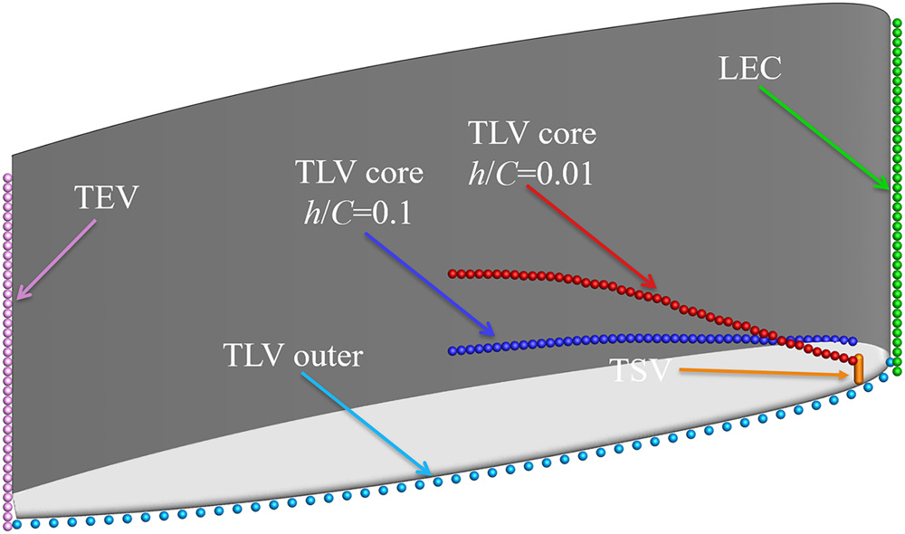
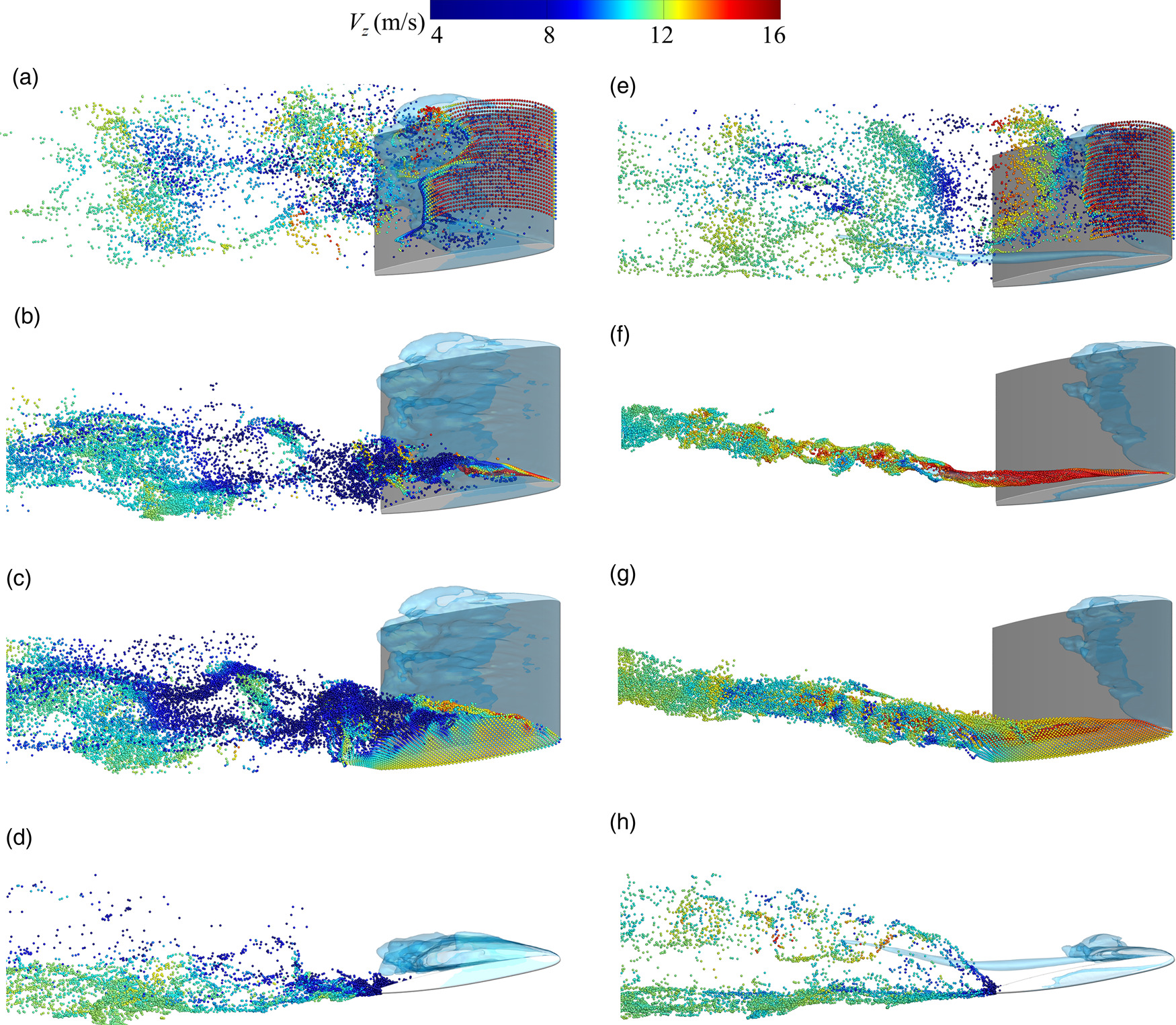
The snapshots of streaklines of flow structures are presented in Figure 15. The fluid particles are colored by instantaneous streamwise velocity. In our previous studies (Hou et al., 2022; Hou and Liu, 2023), the TLV is composed of a two-layer structure, so two sets of seeding points are set in the TLV core and gap. The fluid particles in LEC clearly demonstrate the periodic process of cloud cavitation shedding and re-entrant jet. As shown in Figures 15(c)–15(f), the velocities of fluid particles in the TLV core and outer layer are similar, regardless of the gap size. Only in the generation stage of the TLV, the streamwise velocity of the TLV is relatively high at h/C = 0.01. As discussed before, the losses arising from the tunnel boundary layer is the main factor results in a streamwise velocity deficit in the TLV. This conclusion is consistent with the previous results (Batchelor, 1964). Further, the fluid particles in the TLV at h/C = 0.01 exhibit low-frequency fluctuation due to the effect of LEC periodical development, which may also suppress the vorticity transport related to the TLV. Unlike the TLV that become instability and breaks prematurely at h/C = 0.01, the TLV at h/C = 0.1 is more stable from LE to TE, and shows a jet-like behavior. However, at the downstream of hydrofoil, the TLV at h/C = 0.1 also exhibits slightly instability. Figures 15(g) and 15(h) reflect the influence of TEV on the stability of TLV. It is clearly observed that due to a small distance between the TLV and hydrofoil, the TEV near the gap is captured by TLV at h/C = 0.1. However, the vorticity transport process between the TEV and TLV is weak at h/C = 0.01. It is also found that a portion of the wake flows back to the SS of the hydrofoil, which results from the periodic evolution of large-scale LEC.

Figure 15.

Snapshots of streaklines of flow structures. (a) LEC, h/C = 0.01, (b) LEC, h/C = 0.1, (c) TLV core, h/C = 0.01, (d) TLV core, h/C = 0.1, (e) TLV outer, h/C = 0.01, (f) TLV outer, h/C = 0.1, (g) TEV, h/C = 0.01, (h) TEV, h/C = 0.1.

All the streaklines of complex flow structures are shown in Figure 16. The fluid particles are colored by their release position, according to Figure 12. At small gap size condition, the vorticity transport from tip to the TLV is weak, resulting in an indistinct two-layer structure of the TLV. As the TLV develops, the fluid particles released from the TLV core, TLV outer layer, and LEC are mixed. The particles of the wake are basically located at the bottom of the TLV. As the gap size increases, the two-layer structure of TLV becomes significant. The inner TLV core region is generated by the vorticity transport from the tip to the TLV. The TLV core region corresponds to TLVC, in which no particles released from other structures appears. The structure of the outer layer including the mainstream, TSV and leakage flow, is formed by the shearing between the tip leakage flow and the passage flow. The complex outer layer plays a crucial role in affecting the stability of TLV as well as cavities.

Figure 16.

Summary of streaklines of complex flow structures. (a) h/C = 0.01. (b) h/C = 0.1.

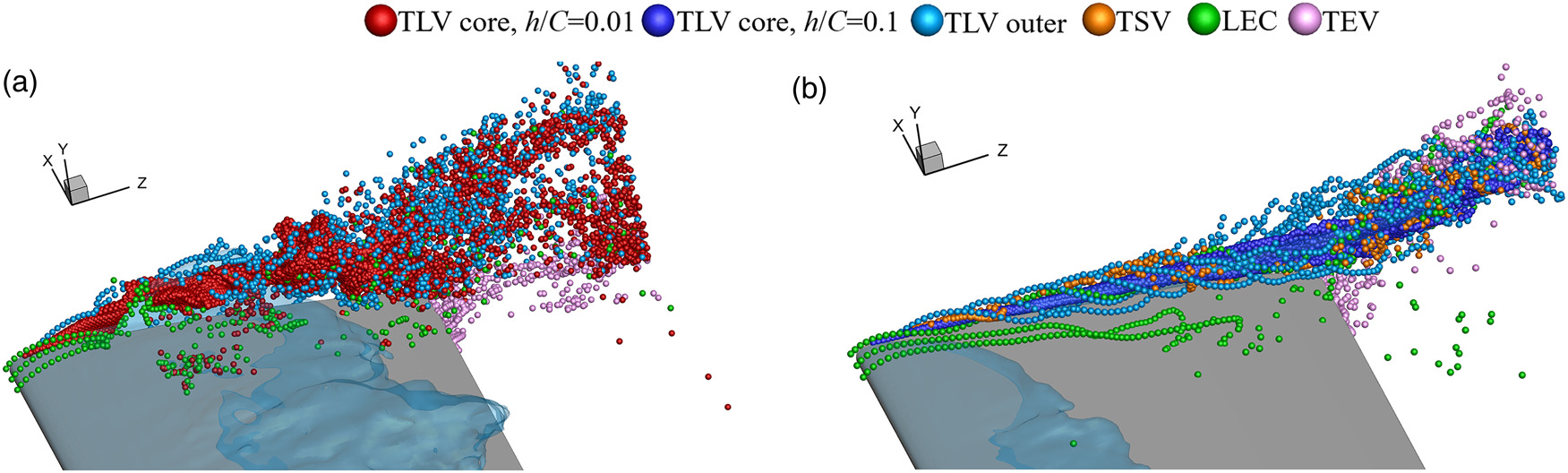
The investigation on TLV structure in this study of cavitation flow is in good agreement with the previous conclusions in compressors (Hou et al., 2022), indicating that two-layer structure of the TLV is a universal phenomenon, providing support for the mechanism research and flow control of the TLVC in the future.