
Introduction
To achieve higher engine efficiency and specific thrust, the single-stage pressure ratio and aerodynamic loading of the compressor are continuously increasing. With the increasing loading, the reverse pressure gradient in the compressor significantly improves in small mass flow conditions. Under these circumstances, the problem of corner separation becomes more severe, leading to reduced working performance of the compressor. This causes a reduction or completely offset of the benefits of increasing the single-stage pressure ratio and loading, necessitating the implementation of flow control methods to inhibit corner separation.
The fillet was originally considered only as a necessary structure for blade processing. However, some scholars have discovered that it can be utilized as a passive flow control method. A theoretical study of the corner boundary layer of the vertical wall, Debruge (1980) proposed that fillet in an appropriate radius could reduce the thickness of the boundary layer at the wall junction, which could theoretically suppress the corner separation of the turbomachinery. NASA (Brockett and Kozak, 1982) conducted the first study on the influence of fillet on the leading edge (LE) of the wing, and discovered that an overall improvement of the flow field could be achieved by applying a specific fillet on the LE. Subsequently, a full fillet experiment (Curlett, 1991) was conducted in a low-speed cascade environment. The findings indicate that fillet can effectively suppress corner separation of the double-circular-arc cascade, decrease flow loss at high angles of attack, and expand the available working range of the cascade. Some researchers (Hoeger et al., 2002) proposed that fillet design can reduce the 3D discharge changes known as under- and overturning. Later (Sauer et al., 2000) the fillet design was used in turbine environment, and the results demonstrate that fillet design on the LE can significantly reduce the end wall loss. Martin conducted numerical simulations of large-scale fillet on low-speed plane cascades, demonstrating the benefits of fillet on stage matching and inlet distortion. A slow-speed wind tunnel cascade test (Müller et al., 2004) was carried out to demonstrate that the appropriate size of the bubble LE and fillet can improve the compressor cascade performance. Later (Hoeger et al., 2006), fillet experiments and numerical studies on low-speed cascades were conducted, revealing that fillet can mitigate corner separation under extreme inflow conditions by reducing the curvature of the LE of the cascade. An experiment (Meyer et al., 2012) was finished to analyse the fillet influence and was found that the fillet smaller than boundary layer thickness could cause static pressure coefficient rise. An innovative compressor fillet blade end wall fusion technology (BBEW) was proposed (Tian et al., 2013) to mitigate or weaken the low energy corner flow of Rotor67. Gao et al. (2016) have also investigated the effect of blade root fillet on the performance of compressor cascade.
However, there are researches that fillets with variable profiles along the axial direction can benefit the flow field and improve the performance. Reutter et al. (2014) presented the optimal variable fillet design results of the NACA65 cascade using a surrogate model. The research results demonstrate the potential of fillet structure to mitigate the separation of the compressor corner region. According to Tang and Ning (2012), Li et al. (2017) and Wang’s et al. (2016) researches, variable fillet does have different influence on cascade performance. Meanwhile, variable fillet (Ananthakrishnan and Govardhan, 2018) shows more performance improvement than uniform fillet in a transonic axial flow turbine stage.
Based on previous researches, scholars have extensively investigated the influence of uniform fillet on the internal flow field and gained profound insights. The factors contributing to the reduction of corner separation includes: 1, attenuation of the leading-edge horseshoe vortex; 2, utilization of the fillet vortex that counteracts the direction of the channel vortex for suppressing flow separation; and 3, altering the spanwise loading distribution, which weakens the wake and decreases wake loss. However, the influence mechanism and design criterion of variable fillet remains not clarified. Therefore, a parameterized variable fillet design method is proposed. The influence on performance and flow mechanism of uniform and variable fillet is illustrated. Unsteady simulation based on SBES intensifies the understanding of the loss and flow mechanisms. This study aims at providing necessary theoretical supports for variable fillet design.
Methodology
Cascade geometry and fillet design method
In this study, the effects of various fillet designs on the aerodynamic performance of the NACA65-K48 cascade are investigated. The NACA65-K48 is a highly loaded cascade that exhibits significant corner separation at large attack angles, and has been previously tested by DLR (Hergt et al., 2011). Table 1 shows the design parameters and test conditions at the aerodynamic design point (DP) of the cascade.
Table 1.
Design parameters of NACA65-K48 cascade.
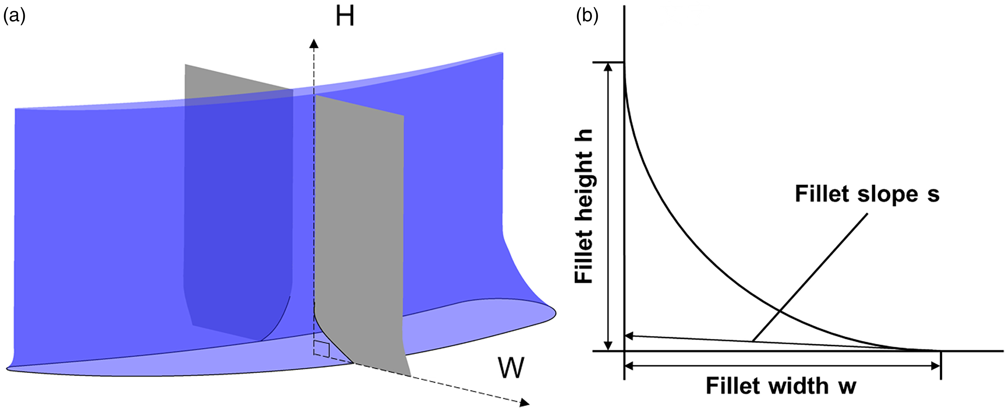
Inspired by Reutter’s work (Reutter et al., 2014), a parameterized variable fillet design method is developed to define the fillet geometry at different axial positions at the pressure side (PS) and the suction side (SS) respectively. At a specific axial position, the fillet shape is controlled by the inverse proportion function determined by three parameters: fillet height (h), width (w), and slope (s), as seen in Figure 1. The control function is given in Equation (1), a, b and c in the equation can be calculated by Equations (2)–(4). Parameter h influences the percentage of passage height occupied by fillet, w influences the passage throat area, and s influences the fillet fullness. Based on the inverse proportion function, the fillet profile at one specific position can be defined by one parameter less than Reutter’s method. For NACA65-K48 studied in this paper, h, w, and s ranges from 0 to 8 mm, 0 to 8 mm, and 0.4 to 100, respectively.
Figure 1.
Fillet configuration and shape control method. (a) fillet configuration (half span), and (b) fillet shape control method at an axial section.
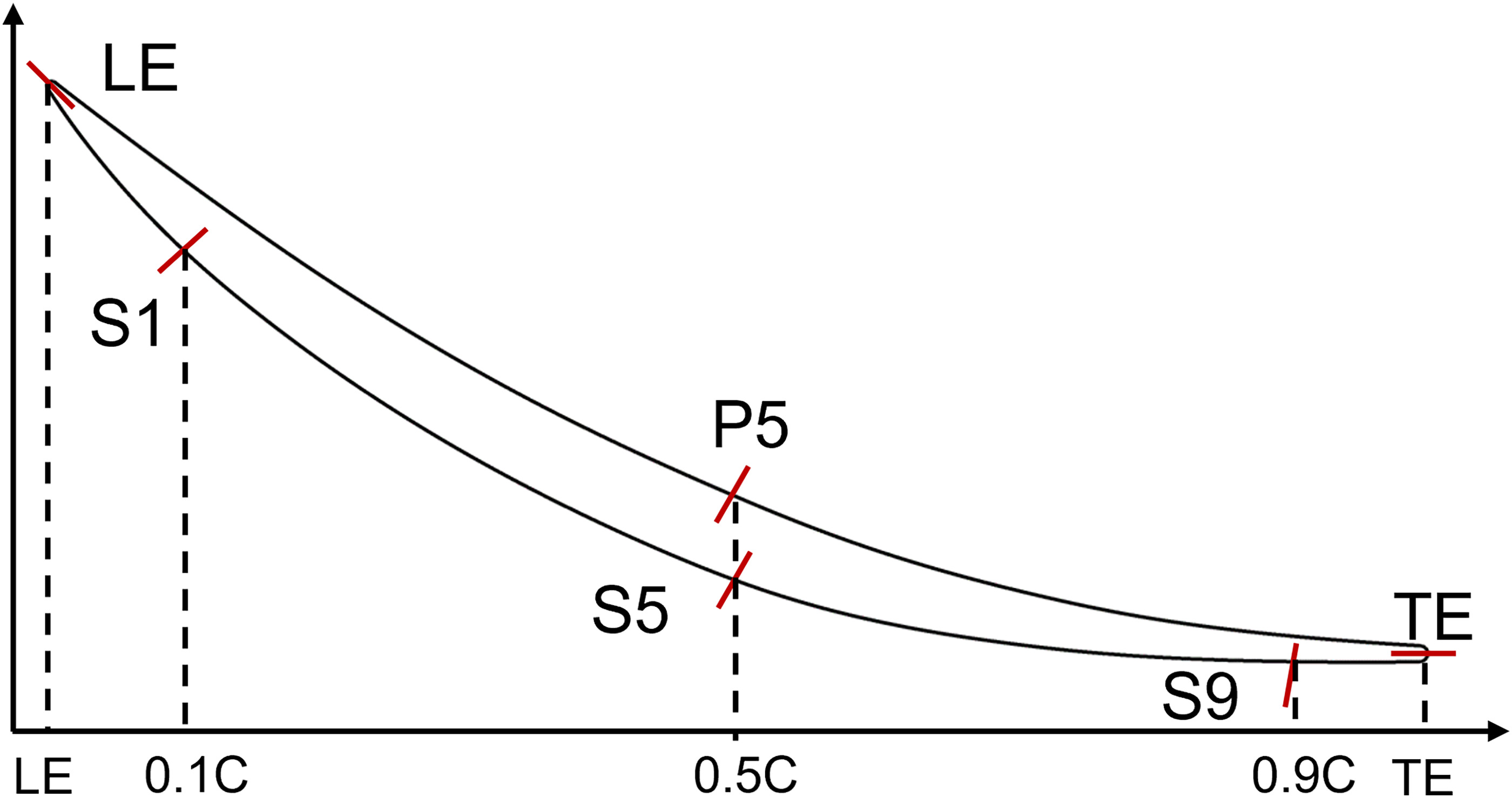
Similar with Reutter’s method, at SS, the fillet profile is controlled by five axial cross sections along the axial direction, including positions at the LE, 10% chord, 50% chord, 90% chord and the trailing edge (TE). Since the fillet at PS shows little influence on the cascade performance, the PS fillet is controlled only by the profile at 50% chord, accompanied with the profiles at LE and TE. The distribution of the fillet control points is shown in Figure 2. To avoid geometric singularity, the parameters at remaining positions are controlled by the B-spline curve fitted by the parameters at positions illustrated. Based on this method, a variable fillet can be defined by 18 parameters on these six sections.
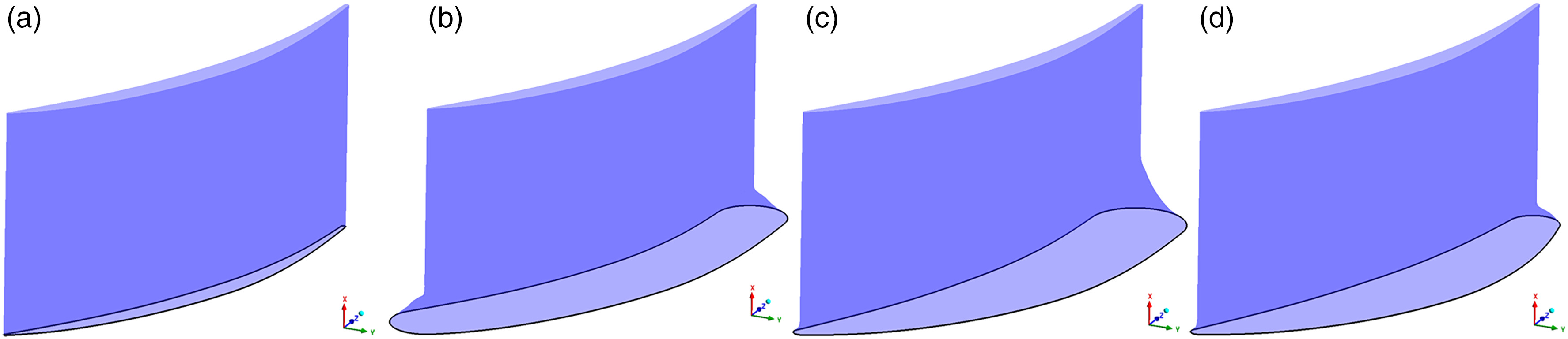
At the preliminary stage, based on the suggestion by Reutter that the fillet size should increase along the axial direction, 300 samples of variable fillets were randomly generated. Among these samples, the fillet configuration that has the best performance improvement on the cascade is named as F_Var in this paper. Except for the cascade without fillet (BASE) and F_Var, two cascades with uniform fillets are generated. One has a uniform fillet size of 0.5 mm (F_0.5), which is the same as the fillet size at the leading edge of F_Var. The other one with a fillet size of 3 mm (F_3.0) has the similar cascade flow path area with F_Var. Besides, two variable fillets with fillet size decreasing after 50% chord are designed to explore the effect of TE fillet size, named as F_Var1 and F_Var2. Geometrical variations produced by these design variables over endwall juncture are visually shown in Figure 3. All these fillet geometries are only applied to one end wall of the cascade while the other end is normal.
Numerical methods and validation
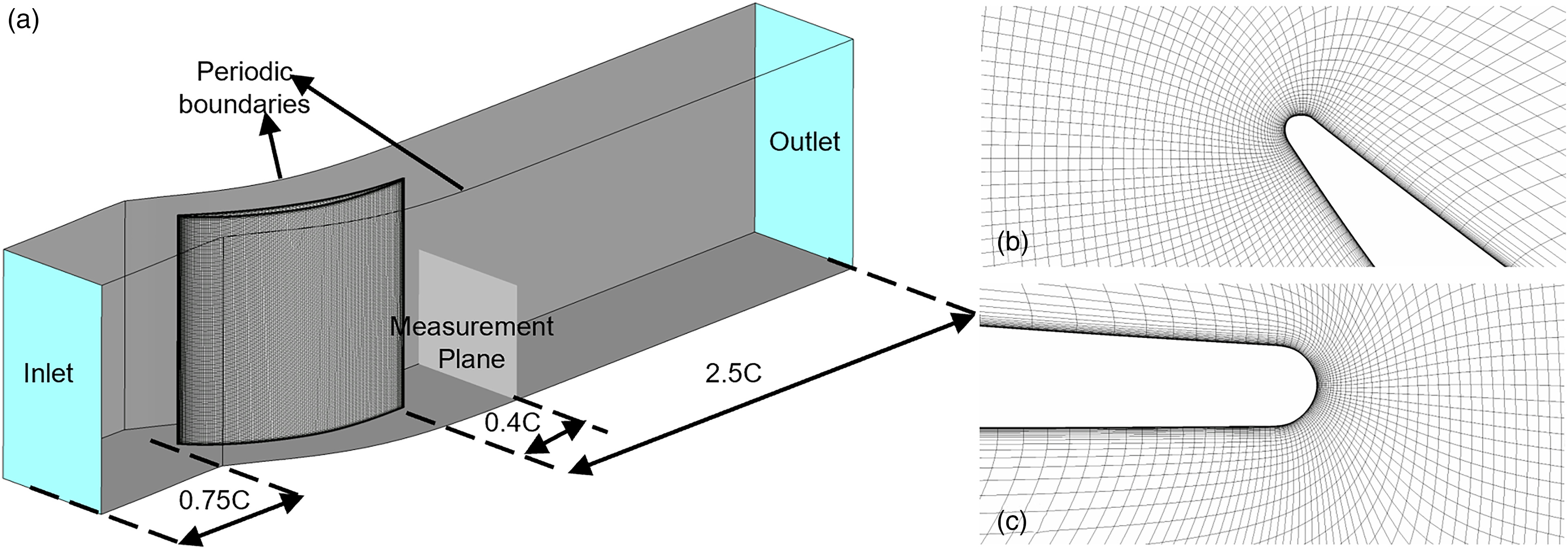
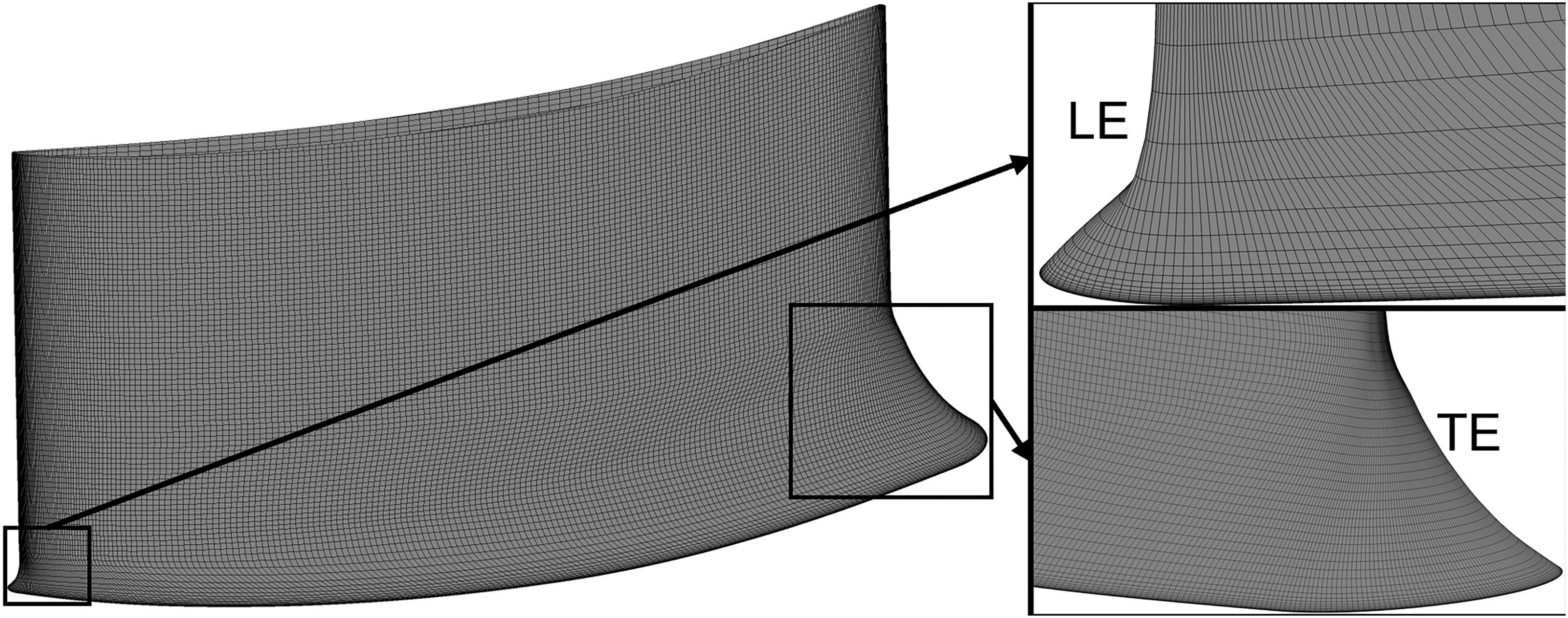
For the flow domain of NACA65-K48 cascade numerically studied in this paper, the inlet plane is extended to 0.75C upstream LE, while the outlet is set to 2.5C downstream TE, as seen in Figure 4(a). The structured grids for the linear cascades are generated by Numeca AutoGrid5 with O4H topology. The mesh topologies at LE and TE are shown in Figure 4(b) and (c). The tangential grid of the cascade is periodically matched. To ensure that the y+ on the blade and end wall is less than 1, the height of the first layer of grid on the wall is less than 1 × 10⁻⁶ m. The cascade performance is measured at the half-span plane 0.4C downstream the cascade, as shown in Figure 4(a).
Figure 4.
Computational domain and mesh topologies. (a) flow domain and boundaries, (b) LE mesh topology, and (c) TE mesh topology.
For cascades with fillets, the fillet and cascade are handled as a whole to generate the mesh. To guarantee mesh quality, minimal mesh topology adjustments are made based on the prototype topology. The mesh details of F_Var are shown in Figure 5 below. It can be seen that the mesh topologies at LE and TE have good quality. Mesh qualities of other cascades with uniform or variable fillets are checked and guaranteed equivalent to BASE as well.
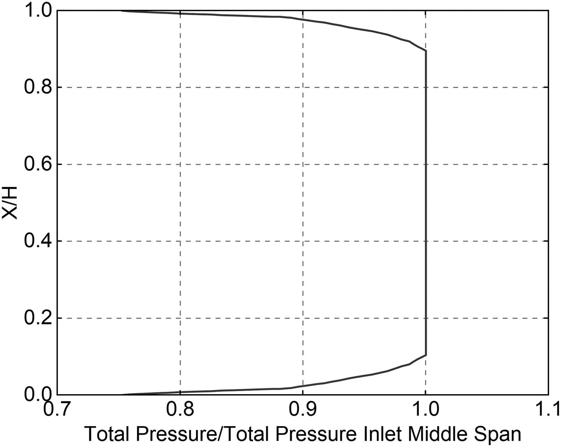
Numerical simulations are carried out by ANSYS CFX 22. The steady simulation employs the Shear Stress Transport (SST) model with gamma theta transitional turbulence, which shows better coincidence with experiment results than that without transitional turbulence. The tangential boundaries are set as translational periodic, while the end walls and the cascade blade are set as non-slip adiabatic wall. A constant total temperature of 322 K, inlet flow angle, and a profile of total pressure derived from experiment are imposed at the cascade inlet, with 5% turbulence intensity. The inlet profile is shown in Figure 6. At outlet, mass flow rate
Grid independence test for BASE cascade is carried out. Four levels of grid are simulated by steady simulations: Grid 1 with 5684079 nodes, Grid 2 with 6986559 nodes, Grid 3 with 10054020 nodes, and Grid 4 with 12110451 nodes. Details of grid settings are given in Table 2. Figure 7 depicts the mass-averaged total pressure loss coefficient ω at 40% chord downstream TE of four grids. The total pressure loss coefficient ω is defined as follow:
where pt represents the local total pressure while pt,∞ and ps,∞ represent total and static pressure at inlet mid-span.Table 2.
Grid settings for independence test.
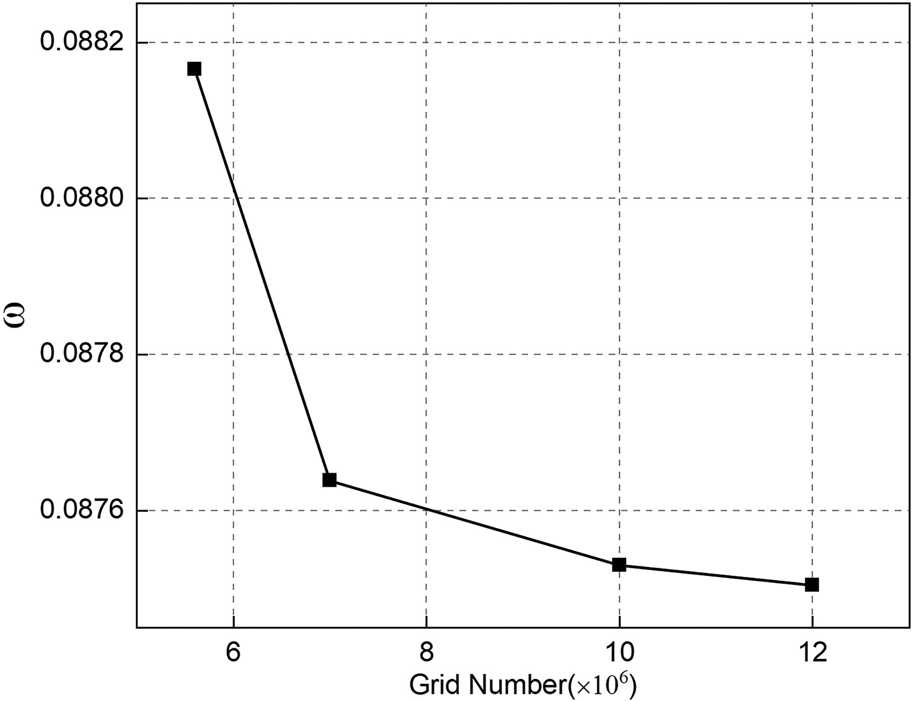
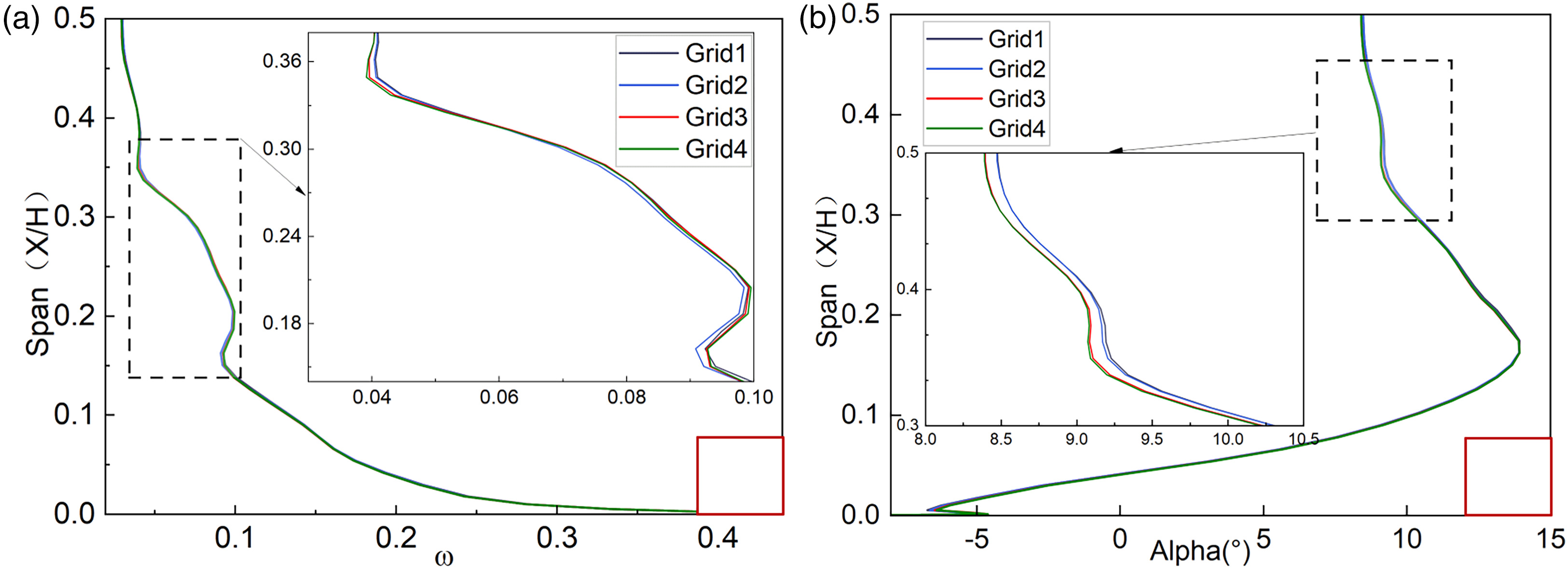
Figure 7 shows that the mass-averaged ω of Grid 2 exhibits variations of 0.4% compared to Grid 1, while the variation between Grid 3 and Grid 2 is 0.1%, and the variation between Grid 4 and Grid 3 is only 0.03%. Figure 8(a) shows that the ω of Grid 1 and Grid 2 differs from Grid 3 and Grid 4 at the 25% to 40% height range. The outlet angle distributions in Figure 8(b) demonstrate that, Grid 1 and Grid 2 show a small difference from Grid 3 and Grid 4 at the 30% to 50% span range. Based on above analysis, Grid 3 is selected for numerical research to obtain more detailed flow field information.
Figure 8.
Effect of grid density on spanwise distributions of aerodynamic parameters. (a) total pressure loss coefficient ω, and (b) outlet flow angle.
For the unsteady numerical simulation, the Stress Blended Eddy Simulation (SBES) model is used as turbulence model. The SBES model is a hybrid RANS-LES method that can switch from RANS to LES model in the transition region by using the shielding function (Menter, 2018). According to our previous work (Lu et al., 2021), the physical time step ΔT is set to be 1 × 10⁻⁶ s, with a corresponding CFL number lower than 1.0. In unsteady simulation, outlet condition is set with the static pressure obtained from the steady simulation results. This type of setting can save time cost while ensuring computational reliability. Additional criteria for judging the convergence include the ratio of the inlet and outlet flow difference to the inlet flow (<5‰) and the average velocity change rate in the corner area monitor point (<5‰).
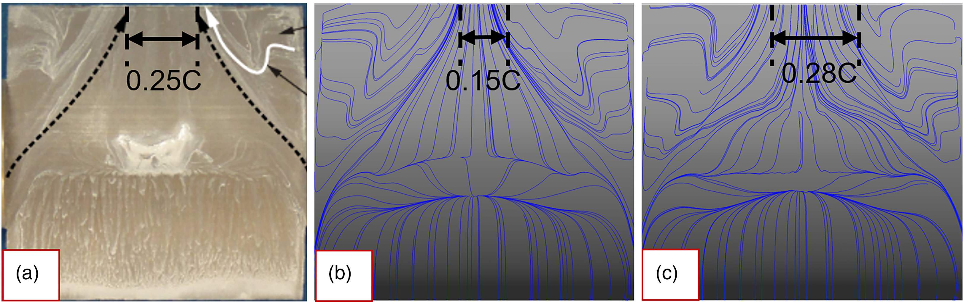
To compare the accuracy of the numerical simulation results with the experimental data and establish their reliability, Figure 9 displays the spanwise distributions of ω and alpha (relative to the axial axis). The limiting streamline results on blade surface are also given in Figure 10. According to the streamline results, it can be seen the main flow take about 0.25C for experiment, 0.15C for RANS results and 0.28C for SBES. These results show advantages of SBES.
Figure 9.
Comparison between experimental and different numerical results. (a) outlet flow angle, and (b) total pressure loss coefficient.
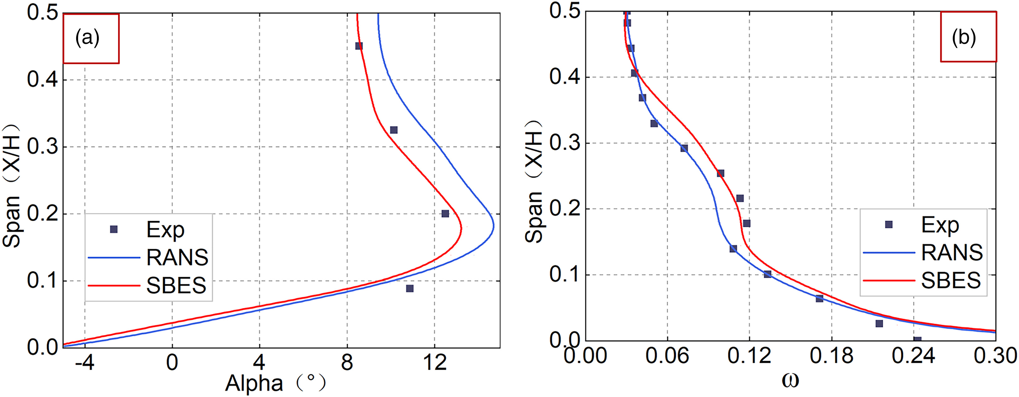
Figure 10.
Distributions of blade surface limiting streamlines. (a) experiment, (b) RANS result, and (c) SBES result.
These findings suggest that RANS turbulence models can predict the general trends while SBES result shows more accuracy in predicting corner separation flow details. Considering the cost of time and the accuracy of calculations, steady RANS simulation based on SST turbulence model with gamma theta transition is used for all cascades at all conditions while unsteady simulations using SBES model were carried out for several chosen cascades at near stall condition.
Results and discussions
Comparisons among uniform fillets and variable fillet
This section aims at expounding the different influence mechanisms of uniform and variable fillets on performance and flow fields. Two uniform fillets F_0.5 and F_3.0 and one variable fillet F_Var are compared. The curves of ω and static pressure coefficient Cp versus attack angles are presented in Figure 11(a) and (b). Cp is defined as follow:
Figure 11.
Performance characteristics of BASE, uniform and variable fillets. (a) total pressure loss coefficient ω, and (b) static pressure coefficient Cp.
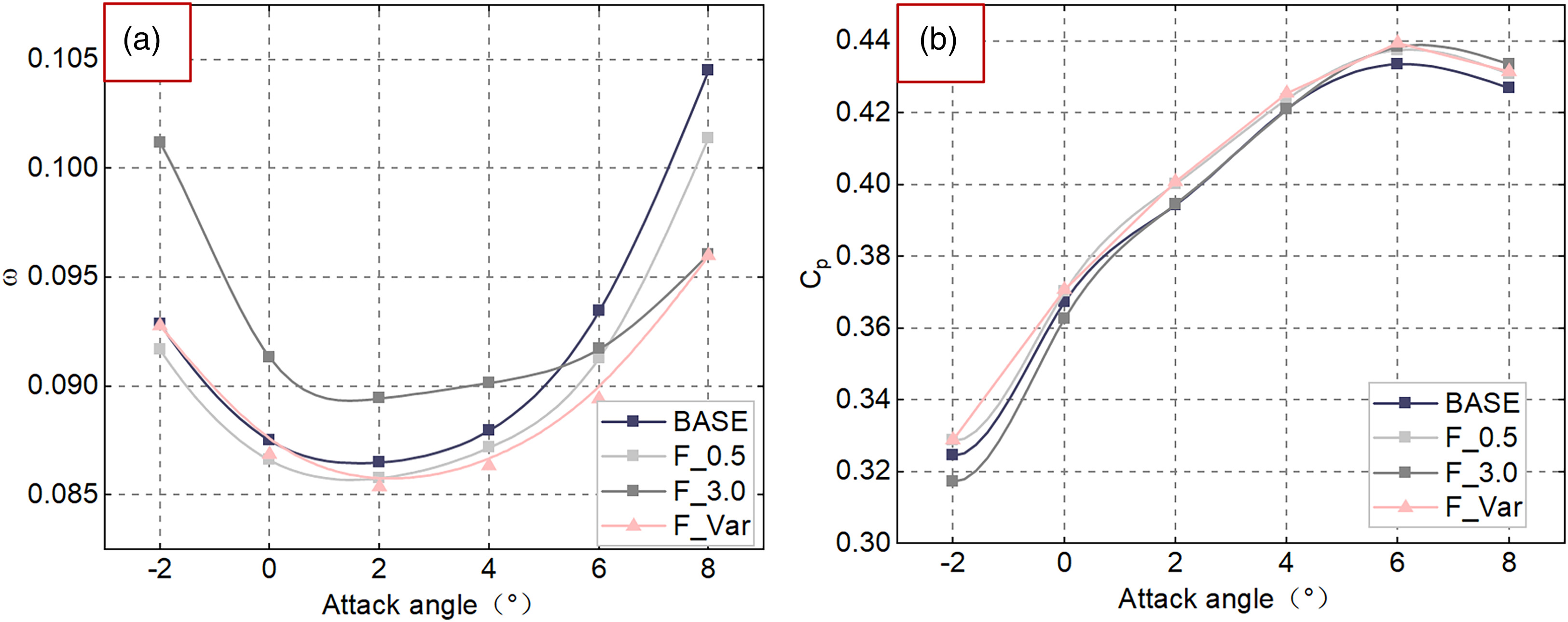
In Figure 11(a), F_0.5 shows slightly reduction of ω at all attack angles, while F_3.0 decreases the loss largely at large attack angle but increases ω when attack angle is less than 5°. As for F_Var, significant reduction in ω is achieved at near stall attack angle (NS), while no additional loss is observed at lower attack angles. This indicates that F_Var has good performance improvement over the entire attack angle range. As seen in Figure 11(b). F_Var and F_0.5 shows similar ability in improving Cp over the entire range, while F_3.0 can improve Cp at NS while decrease Cp near DP.
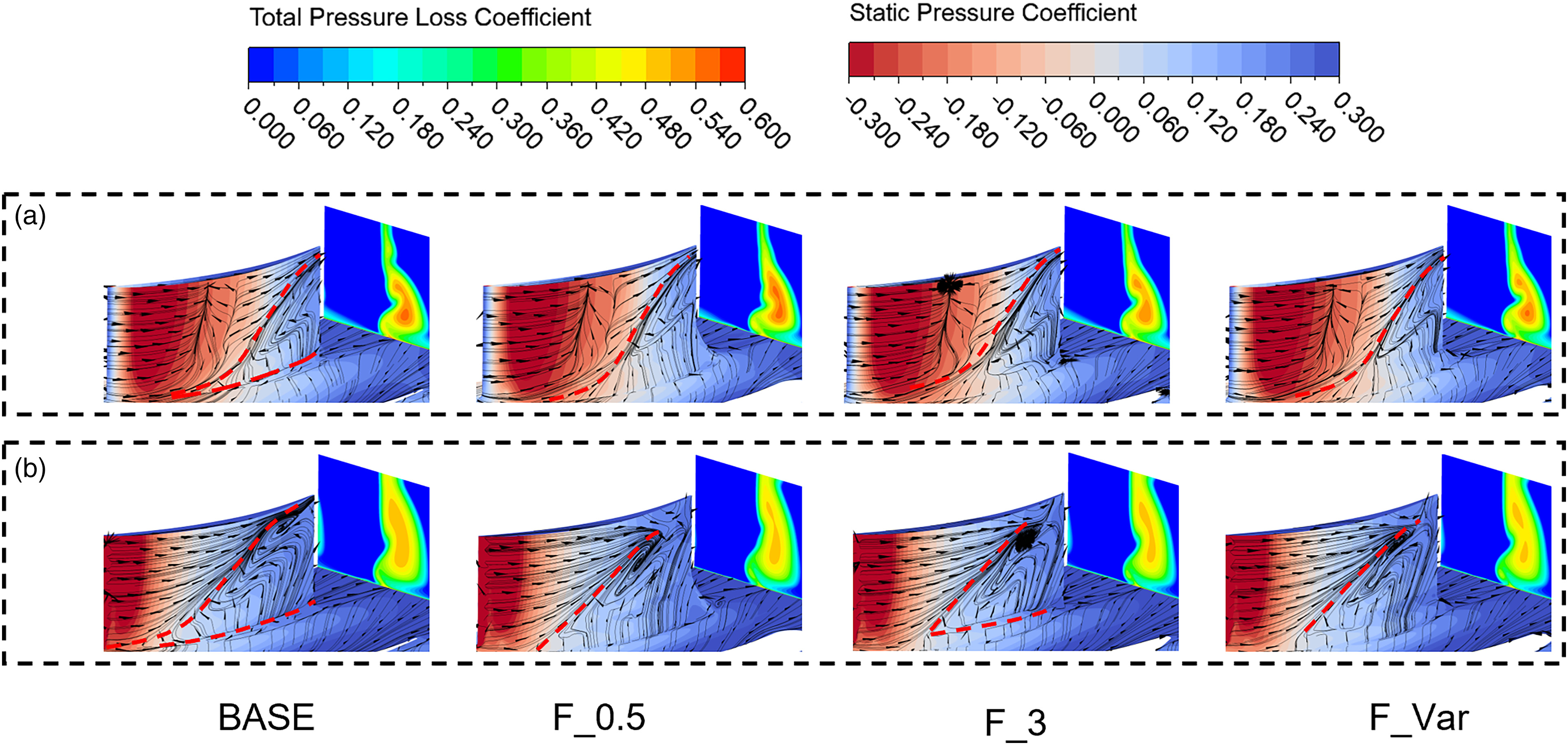
To deepen the understanding towards the fillet influence mechanism, DP (0° attack angle) and NS (8° attack angle) conditions are chosen for following detailed analysis. The distributions of ω downstream TE and Cp at surface at DP and NS are depicted in Figure 12, accompanied with limiting streamlines (Only the range below 50% span is presented).
Figure 12.
Comparisons of total pressure loss, static pressure coefficient, and limiting streamlines. (a) DP condition, and (b) NS condition.
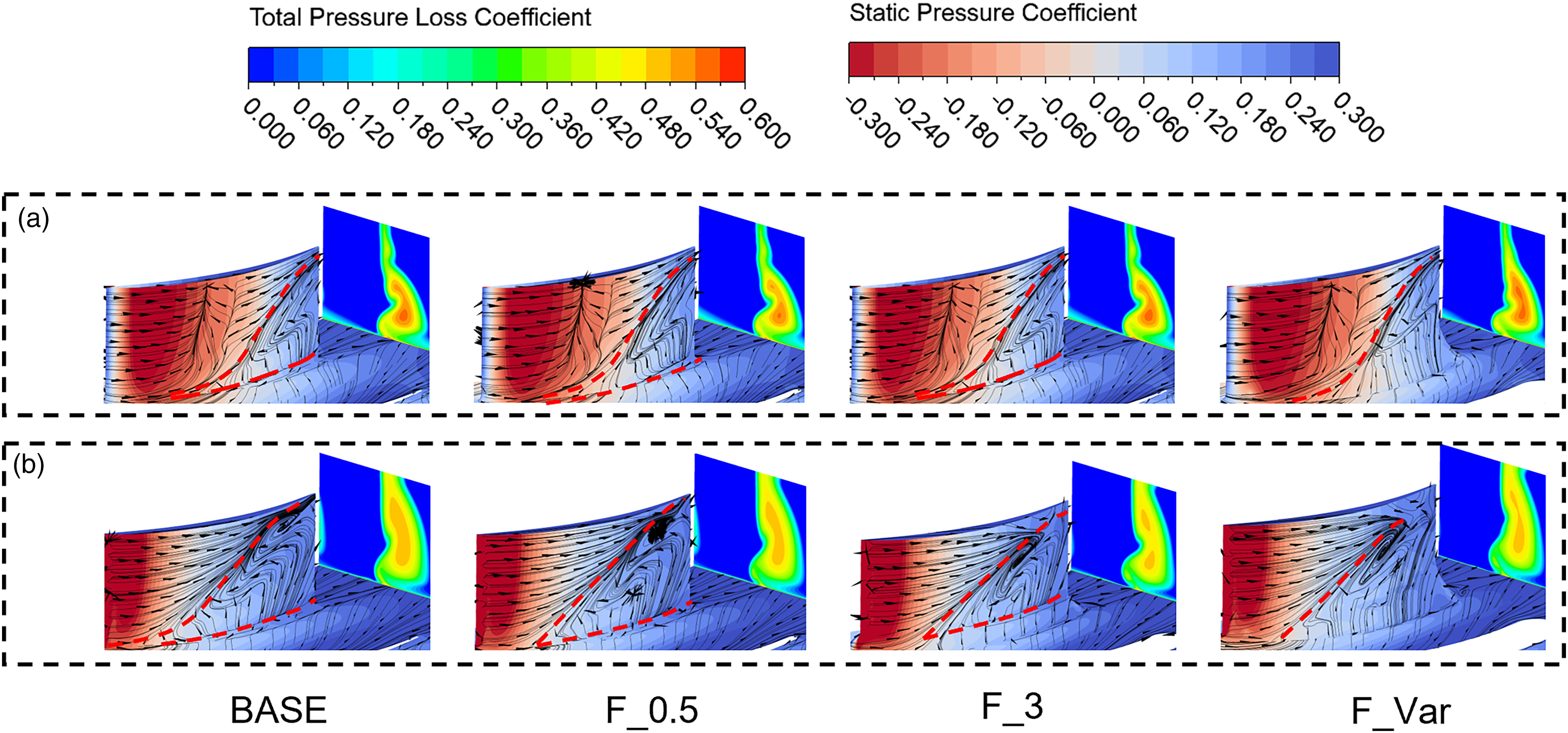
For BASE, there are corner separation regions at both conditions. The reverse flow region starts at about 10% span and 50% axial chord at DP. F_0.5 barely contributes to improvement to the outlet and endwall flow fields. Different from F_0.5, F_3.0 shows an obvious increment of loss core. The F_Var leads to 5% increase in height and 5% axial delay of the chord for the starting position of the reverse region, resulting in an elevation of the high loss region. Besides, the small corner separation region near the end wall is eliminated, since the 3 mm fillet occupies the corner region. At the NS condition, F_0.5 does not show obvious influence on the flow fields, while F_3.0 greatly decreases the high loss region.
F_Var shows a significant reduction in loss within the core region, which can be attributed to both the shrinking of the corner region and restriction of reverse flow. By comparing the Cp distributions, it can be seen that F_0.5 shows the ability to slightly change the Cp distribution near the TE on DP condition, but it has no obvious impact at NS condition. F_3.0 can produce similar Cp distribution influence with F_Var on hub, but it generates a different high-pressure region near corner region, which would deteriorate the local corner flow. F_Var results show that the transverse pressure gradient is notably increased under both conditions. This effectively eliminates the low velocity region at the corner, while simultaneously causing the streamline node to shift upstream from BASE due to an increment in reverse pressure gradient.
The contours of axial wall shear and limiting streamlines are shown in Figure 13. Similar with the spanwise wall shear distributions, F_0.5 hardly changes the axial wall shear at both conditions, while F_3.0 lifts the axial separation region upward, exceeding 50% blade height at DP condition. While at NS condition, the reverse flow region is smaller than BASE and F_0.5. The influence trend of F_3.0 on the axial separation zone is consistent with the loss distribution at different angles of attack in Figure 11. As for F_Var, the axial separation regions near the corner are significantly reduced both at DP and NS conditions. This also explains why the losses of F_Var are reduced under different attack angles. In addition, it is worth noting that due to the large size of the fillet at the F_Var TE, a significant negative axial shear region appears at the TE fillet. This indicates additional separation occurring, which causes extra losses downstream. This also inspired us to explore whether reducing the fillet size near TE could further reduce the loss.
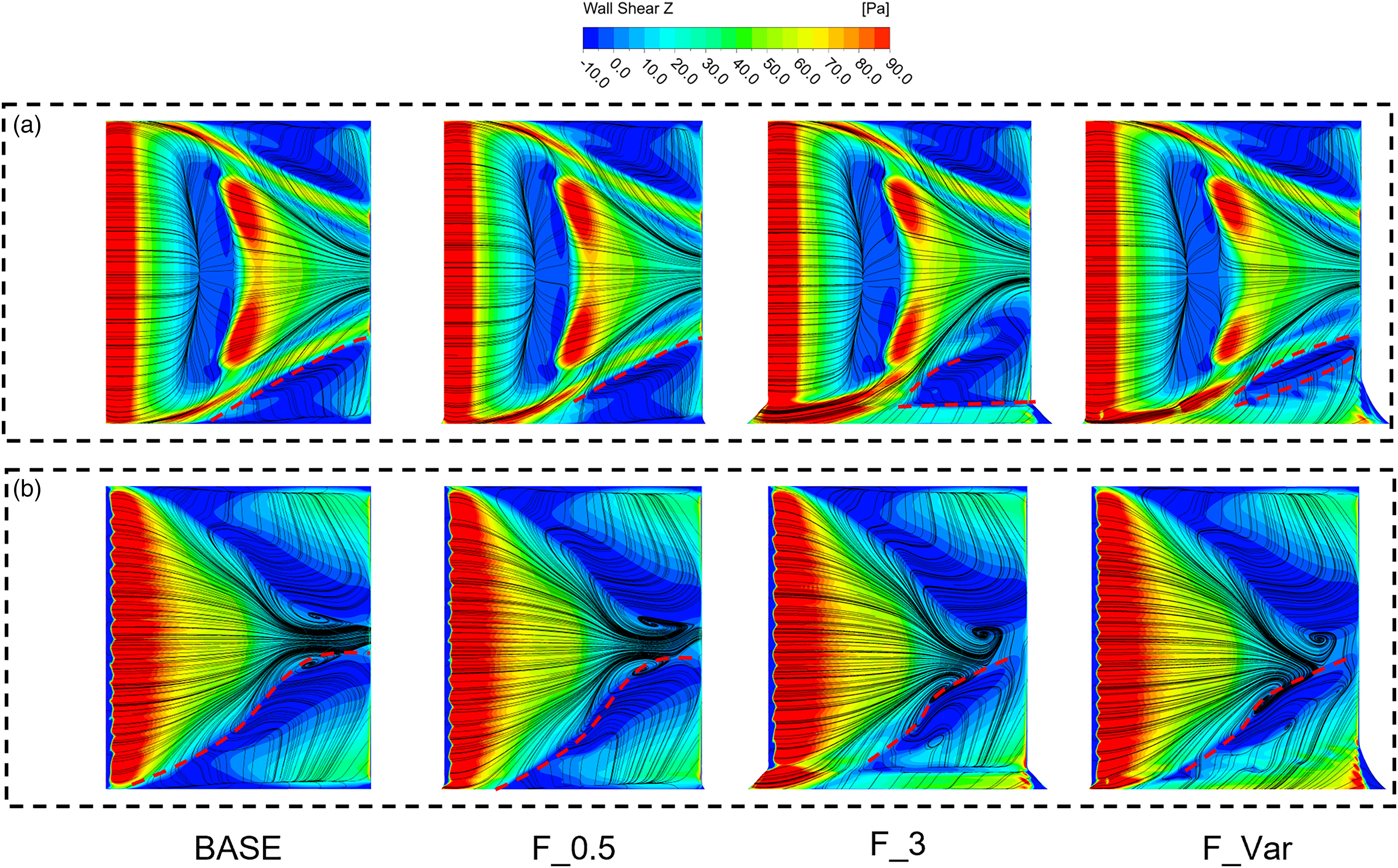
Effects of variable fillets with decreasing size towards TE
Based on the analysis above, it can be seen the F_Var shows different influence mechanism with F_0.5 and F_3.0. F_Var has the ability in restraining corner reverse flow and eliminating the end wall separation, which benefits the flow field and cascade performance. Since the fillet size increases from LE to TE, the fillet at TE causes additional reverse flow and does harm to the flow fields. According this finding, other two variable fillet with decreasing fillet size from mid-chord to TE are designed and investigated. Cascade with fillet increases from LE to 50% axial chord and decreases later is named as F_Var1. The fillet size of F_Var1 is the same as F_Var before the 50% chord length, and after 50%, the size is symmetrically distributed with 50% chord as the centre. F_Var2 has the same distribution of fillet size before 50% chord, and decrease slowly to reach a h and w of 2 mm at TE.
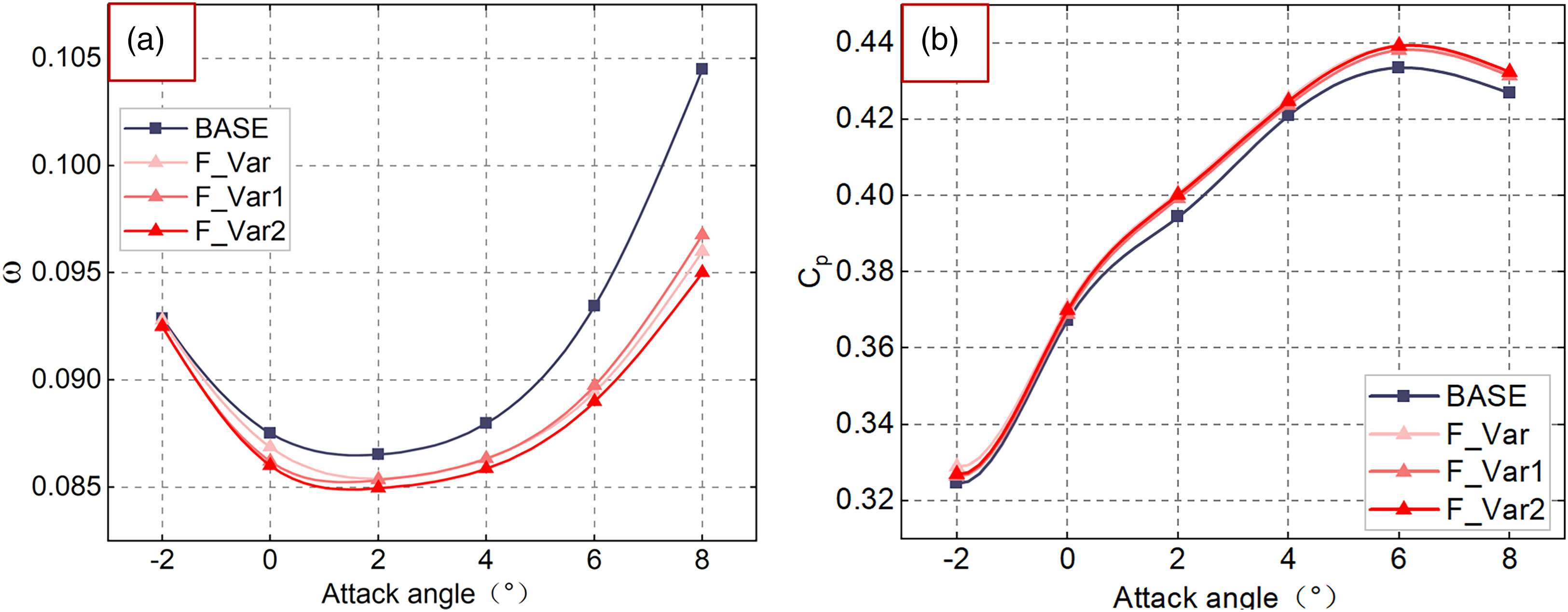
It is noticeable that although the ω performance improves at all attack angle for different variable fillet, F_Var2 shows the best performance improvement, as seen in Figure 14(a). In Figure 14(b), F_Var1 and F_Var2 keep similar static pressure-rise ability with F_Var, while all geometry show improvement. DP and NS conditions for these cascades are chosen for following flow field details analysis.
Figure 14.
Performance characteristics of BASE and variable fillets. (a) total pressure loss coefficient ω, and (b) static pressure coefficient Cp.
The surface limiting streamlines and contours of the ω and Cp are shown in Figure 15. Compared with BASE and F_Var, F_Var1 and F_Var2 all show ω decrease at both conditions. It is clear that at DP, the highest loss on the high loss region decreases for F_Var1 and F_Var2, and the high loss region shrinks noticeably at NS. The Cp distributions do not show an obvious difference, which means that the loadings of these cascades are similar. Based on the limiting streamlines, the reverse flow on F_Var1 and F_Var2 behind TE weakened compared to F_Var. This is the reason for further performance improvements.
Figure 15.
Comparisons of total pressure loss, static pressure coefficient, and limiting streamlines. (a) DP condition, and (b) NS condition.
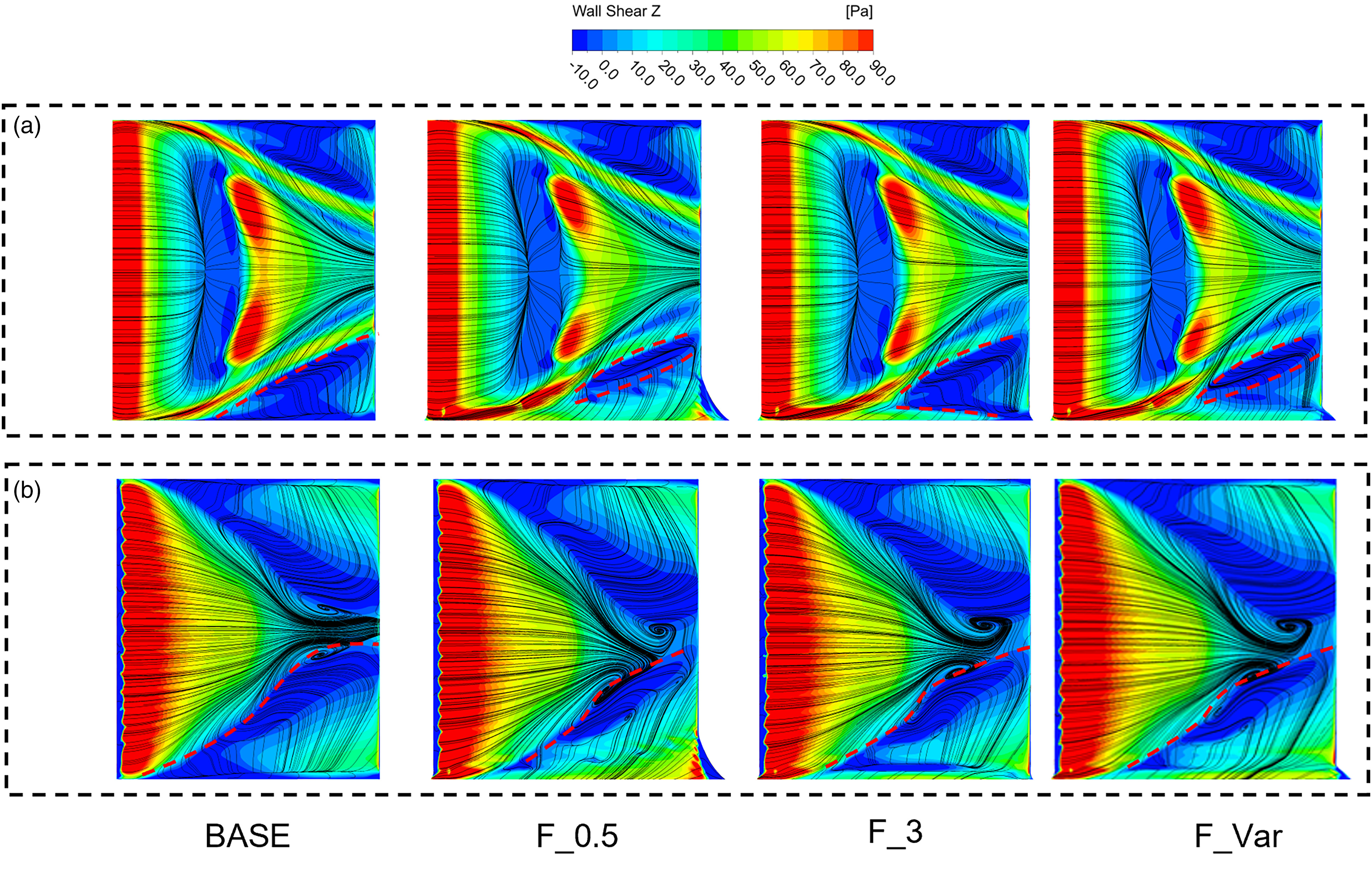
The distributions of spanwise wall shear and axial wall shear are shown in Figure 16, accompanied with surface limiting streamlines. In Figure 16, it is clear that F_Var2 shows more obvious influence than F_Var1 at DP condition, while both F_Var1 and F_Var2 show less influence than F_Var. However, the reverse region areas on end wall TE decrease for both geometries, which benefits the reduction of ω. At NS condition, F_Var2 shows similar influence on blade wall shear with F_Var. F_Var2 also decreases the reverse region areas on end wall TE, which contributes to lower ω than F_Var at this condition.
Figure 16.
Comparisons of axial wall shear and surface limiting streamlines. (a) DP condition, and (b) NS condition.
Based on the analysis above, it can be seen that F_Var, F_Var1 and F_Var2 can significantly improve the cascade performance by influencing the corner low velocity region and reverse flow region. In order to obtain more flow field details and deepen the understanding of the mechanism of influence, BASE, F_Var and F_Var2 are chosen for further unsteady simulations and analysis.
Flow mechanisms of variable fillets restraining corner separation
In order to explore how the variable fillets influences the flow fields, the iso-surface of axial velocity = 0 are plotted to represent the blockage region of corner separation in Figure 17, coloured in helicity Hn, which is defined as follow:
Figure 17.
Comparisons of total pressure loss, static pressure coefficient, and block region. (time-averaged unsteady results). (a) BASE, (b) F_Var, and (c) F_Var2.
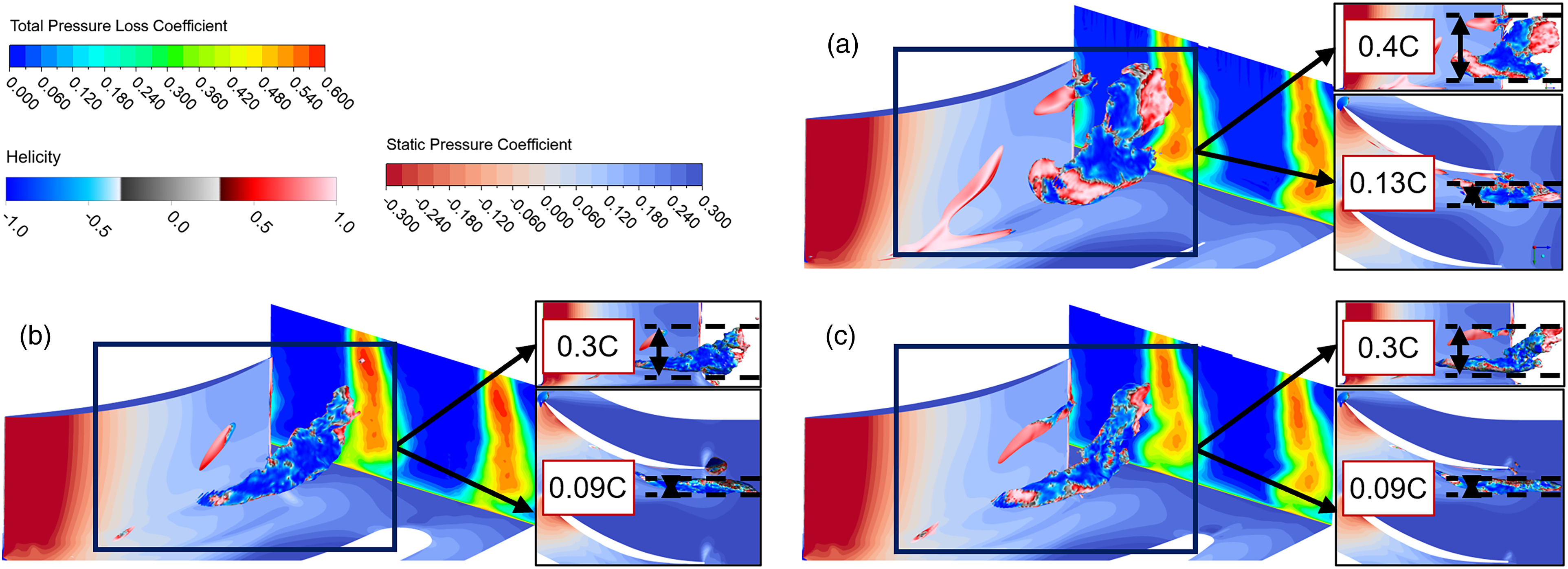
The distributions of Cp on blade and hub and ω at outlet are also presented. Observe the blockage region on BASE, it can be seen the region takes 0.4C spanwise and 0.13C tranverse range. For F_Var and F_Var2, the regions take 0.3C spanwise and 0.09C tranverse range, both show obvious decrease. Meanwhile, the ω distribution shows corresponding decrease. According to the pressure distributions, F_Var and F_Var2 contribute to lower transverse pressure gradient than BASE. Further comparison between F_Var and F_Var2 shows that, the blockage regions within the passage are similar, while F_Var has another small blockage region near the TE. This TE blockage region is consistent with the negative axial wall shear at TE as seen in Figure 16(b) and (c) For F_Var2, this region almost disappears.
Figure 18.
Comparisons of static pressure coefficient, block region and streamlines. (time-averaged unsteady results). (a) BASE, (b) F_Var, and (c) F_Var2.
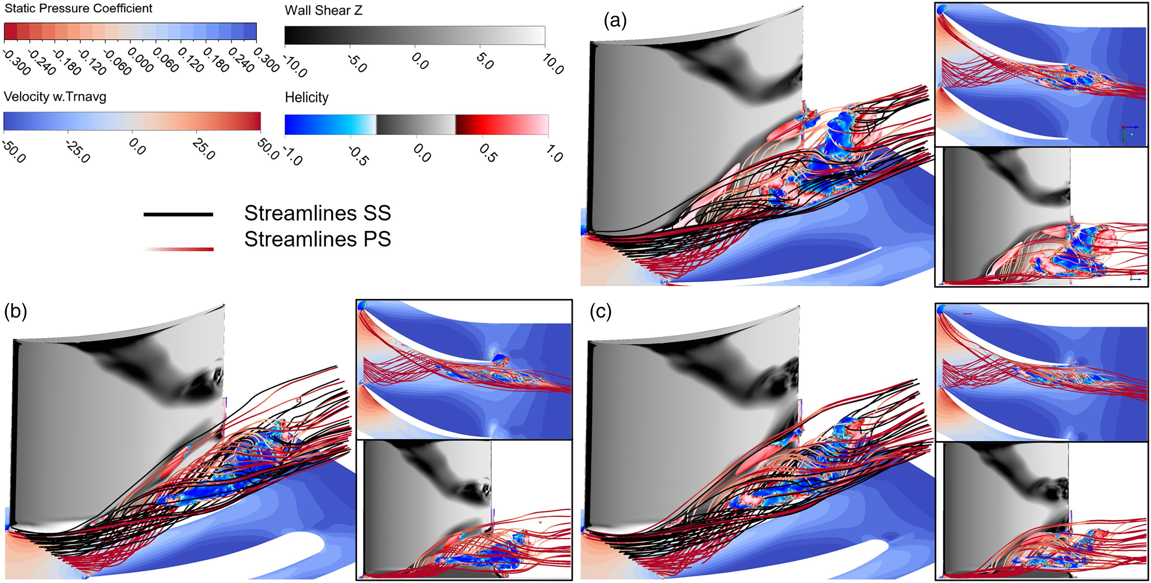
To further illustrate the corner flow evaluation, streamlines from suction side (black) and pressure side (colored in axial velocity) are depicted in Figure 18 respectively. Meanwhile, the axial wall shear distributions are presented at the blade surfaces, as well as Cp distributions at end wall.
According to the results, there are reverse axial wall shear regions for all three cascades. BASE shows the largest reverse axial shear region, while F_Var and F_Var2 shows smaller regions. The reverse flow regions of F_Var and F_Var2 starts further downstream from LE. The streamlines originating from adjacent cascade PS show great consistent with axial wall shear distribution. In the BASE case, SS streamlines, i.e. the black lines, separates near the suction side and forms the largely blockage. Under the strong transverse pressure gradient, the PS streamline flows towards the adjacent blade suction surface, passes from below the SS streamline, flows towards the suction surface and separates. This separated flow together with the SS separated flow forms the large-scale blockage area. As for F_Var and F_Var2 cases, the variable fillet contributes to smaller separation regions caused by SS streamlines. Moreover, due to the decrease of pressure gradient, the PS streamline does not form significant wall separation flow after flowing towards the adjacent blade suction surface. Instead, PS streamlines are involved in the SS blockage and flow out of the passage. Thus, the blockage regions in F_Var and F_Var2 cases are remarkably smaller than that in BASE case.
Based on the results of unsteady SBES simulation, it was found that using variable fillet can effectively reduce the transverse pressure gradient and prevent flow from PS from generating a larger blockage region. Besides, by incorporating a variable fillet with smaller TE fillet size, it is possible to eliminate the additional separation at TE and reduce ω further.
Conclusions
The highly-loaded cascade NACA65-K48 was taken as the research objects. To analyse the influence mechanisms of variable fillet on cascade performance and get the fillet design criterion, a parameterized variable fillet design method was developed and RANS simulation based on SST turbulence model and URANS simulation based on SBES model were carried out. The main conclusions are drawn as follows:
For a uniform fillet, the effect of small fillet (0.5 mm) on performance is limited, while larger uniform fillets (3 mm) can only reduce losses at high incidence angles, and the increase in losses at low incidence angles is significant. Non-uniform fillets have the potential to improve blade performance throughout the entire range of incidence angles. The cascade F_Var2, which has the increasing and slowly decreasing fillet sizes, can decrease the total pressure loss under all attack angle conditions most apparently.
According to the distributions of axial and spanwise wall shears at suction surfaces, the uniform fillet can lift the separation area upward as a whole. But its inhibitory effect on large-scale separation flow only appears at NS condition. The variable fillets can eliminate the small separation near the endwall and significantly reduce the large-scale corner separation, contributing to the loss reduction over the entire operating range. However, the large fillet size at TE will contribute to an additional TE separation and corresponding total pressure loss. Therefore, the fillet configuration with increasing then decreasing size has a greater potential for improving performance.
The SBES unsteady simulations can predict the performance of NS conditions similarly to steady results with SST-gamma theta transitional turbulence. It can be concluded that using a variable fillet can significantly decrease the separation area in the corner. This is due to two main reasons: First, the smooth transition between blade and endwall can reduce the corner separation caused by the SS streamlines; second, the variable fillet can reduce the transverse pressure gradient. Therefore, the PS streamline can flow out of the passage at a higher velocity, without forming additional separation region after arriving the adjacent suction surface.