
Introduction
The performance of the aircraft is directly and inseparably linked to the performance capability of the propulsion system. For this reason, continuous efforts are made to improve the power-to-weight ratio (Kappler, 1981) and ensure high reliability and efficiency for long-term aircraft operation (Wensky et al., 2010). These continuous requirements ultimately result in engine architectures that operate ever closer and with smaller margins to the aerodynamic, thermal, and structural limits of the various engine components. Furthermore, the turbofan engine plays a significant role in future aviation (Mistry et al., 2016; Bowman et al., 2018; Sahoo et al., 2020). The parallel hybrid-electric turbofan engine, as illustrated in Figure 1, poses a significant challenge to the thermal cycle due to its combination of electric power and gas turbine to drive the low-pressure spool. Due to the availability of robust measurement technology and the thrust proportionality, the
The significant limits on the performance of turbofan engines are determined by the material characteristics of the high-pressure turbines (HPT) (Boyce, 2012) and by the distance to the stability limit (surge margin, SM) of the high-pressure compressor (HPC) (Gravdahl and Egeland, 2012). In addition, the hybridisation of a conventional turbofan engine results in a higher load of the low-pressure compressor (LPC). Hence, the operation line of the LPC of a parallel hybrid-electrical turbofan engine is relocated closer to the LPC stability line (Thomas et al., 2018). To ensure safe operation of the turbofan engine, it is of utmost importance that the limits of their performance are not exceeded even under extreme conditions, such as rapid power increases in emergency situations. During such time-dependent manoeuvres, the unsteady behaviour of the engine performance is characterised by an increase in aerodynamic loads, which is attributed to various factors, primarily the inertia of rotating components and secondary effects such as heat transfer, material expansion, and gas dynamics (Walsh and Fletcher, 2004).
During the process of transitioning an aircraft engine from one steady-state operating point to another, it is achieved by means of manipulating the thrust lever position. By increasing the thrust demand, an acceleration is induced through the engine’s the electronic engine control (EEC) which increases fuel flow, thereby increasing temperatures in the combustion chamber (CC). Initially, the high-pressure turbine (HPT) downstream of the CC experiences an energy overflow, while the high-pressure compressor (HPC) upstream is throttled by the temperature increase. Due to the inertia of the rotating components, which transfer energy from the HPT to the HPC, initially no increase in rotational speed is observed during acceleration due to the power imbalance, but primarily leads to a shift of the operating point of the HPC towards the stability limit due to the increased back pressure (primary effect). This reduces the core mass flow and, together with the increased fuel flow, leads to a rapid increase in the fuel to air ratio (FAR) and temperature in the combustor. This example shows that there are aerothermodynamic interdependencies between the operating performance of the components. Meanwhile, unsteady secondary effects also affect the system performance. Heat fluxes are caused by the discrepancies between material and gas temperatures, while the volume storages in the gas path are filled and emptied with gas in a time-dependent manner. The interaction of the secondary effects with the aero- and thermodynamics determines the overall system performance.
The nonlinear and time-dependent system performance motivates the investigation and numerical modelling of the parallel hybrid-electric turbofan engine in this work. Although the influence of primary and secondary effects of the engine has been sufficiently explored (Fiola, 1993; Walsh and Fletcher, 2004; Rick, 2013; Kurzke and Halliwell, 2018), the aerodynamic interdependencies of these effects on each other are only inadequately investigated. This leads to the following research question:
What is the extent of the influence of aerothermodynamic interdependencies of unsteady secondary effects on performance-specific and safety-relevant quantities?
To answer this question, the time-dependent performance of a parallel hybrid-electric turbofan engine is simulated. For this purpose, two different approaches are used: (1) the constant-mass flow (CMF) method and (2) a dynamic approach. In this study, the dynamic approach is able to consider the aerothermodynamic interdependencies. Therefore, the parallel hybrid-electric turbofan engine and its associated performance models will be briefly introduced at the beginning of this study. Following that, the aerothermodynamic interdependencies will be defined and the impact of other secondary effects such as heat transfer on these interdependencies will be analysed. Lastly, the impact of hybridisation will be considered and the results are summarised in the conclusion.
Methods
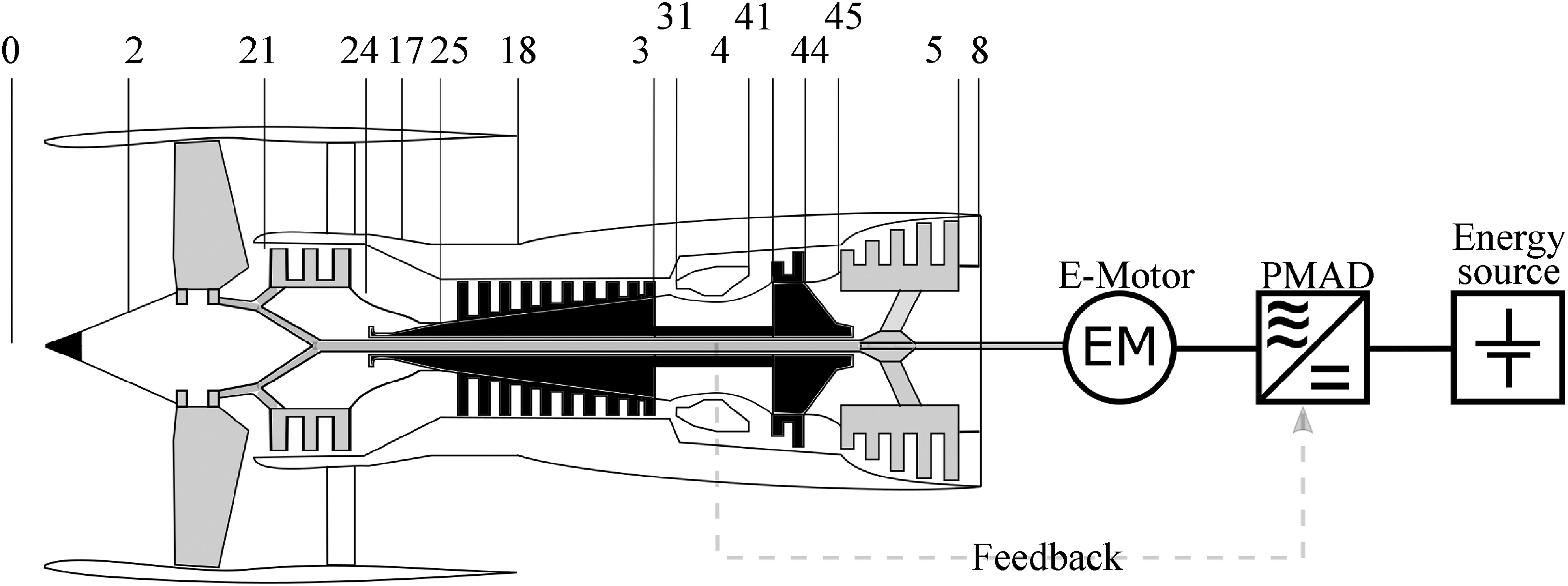
In this study, the International Aero Engines V2500-A1 is used, which is operated on the A320-200 Figure 1 shows the schematic sectional view of the V2500-A1 engine and its corresponding stations.
Figure 2.
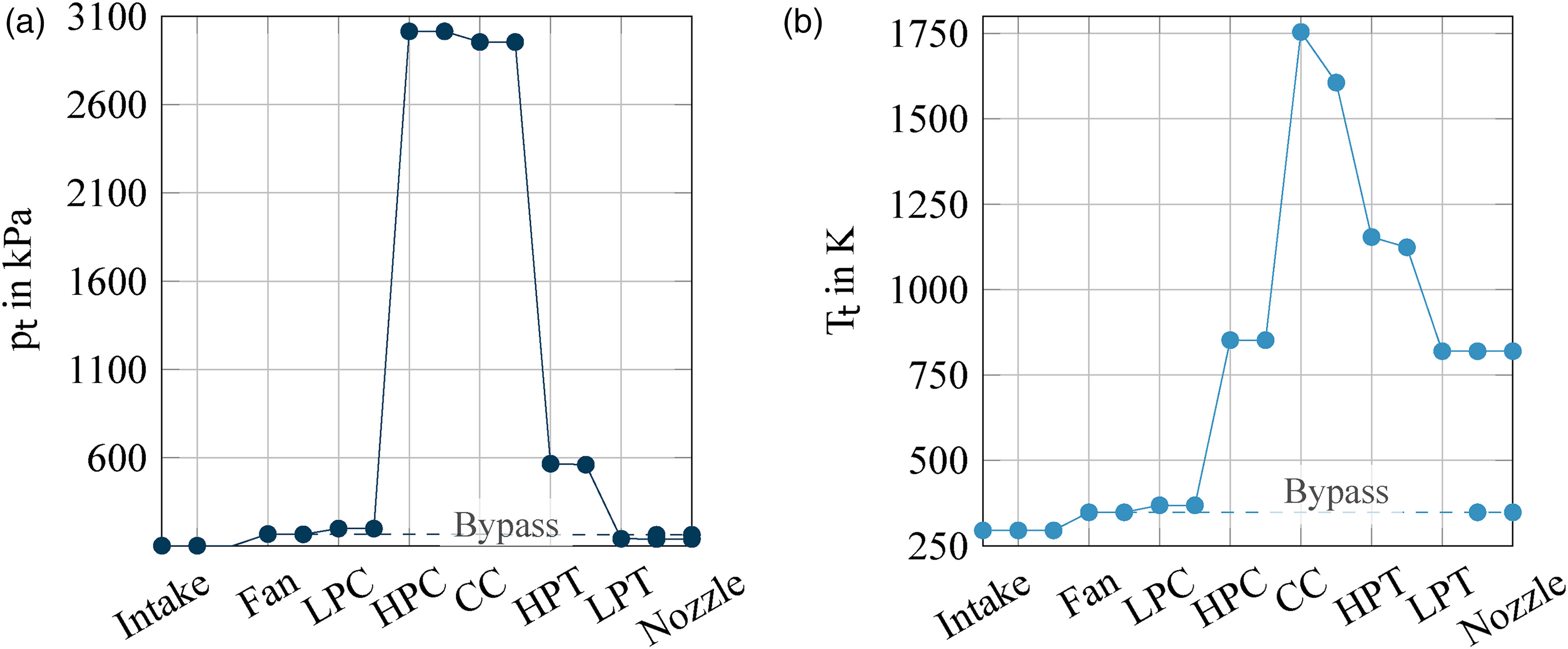
Pressures and temperatures within the turbo components at the takeoff operating point of the conventional aircraft engine.
Hybridisation and electric machine
Due to the hybridisation of the
The power management and distribution (PMAD) system, responsible for distributing power to electrical equipment such as controls, inverters, and cables, is modelled at a constant efficiency of 97%. The efficiency of the electric machine in converting from electrical to mechanical energy is plotted against speed N and torque
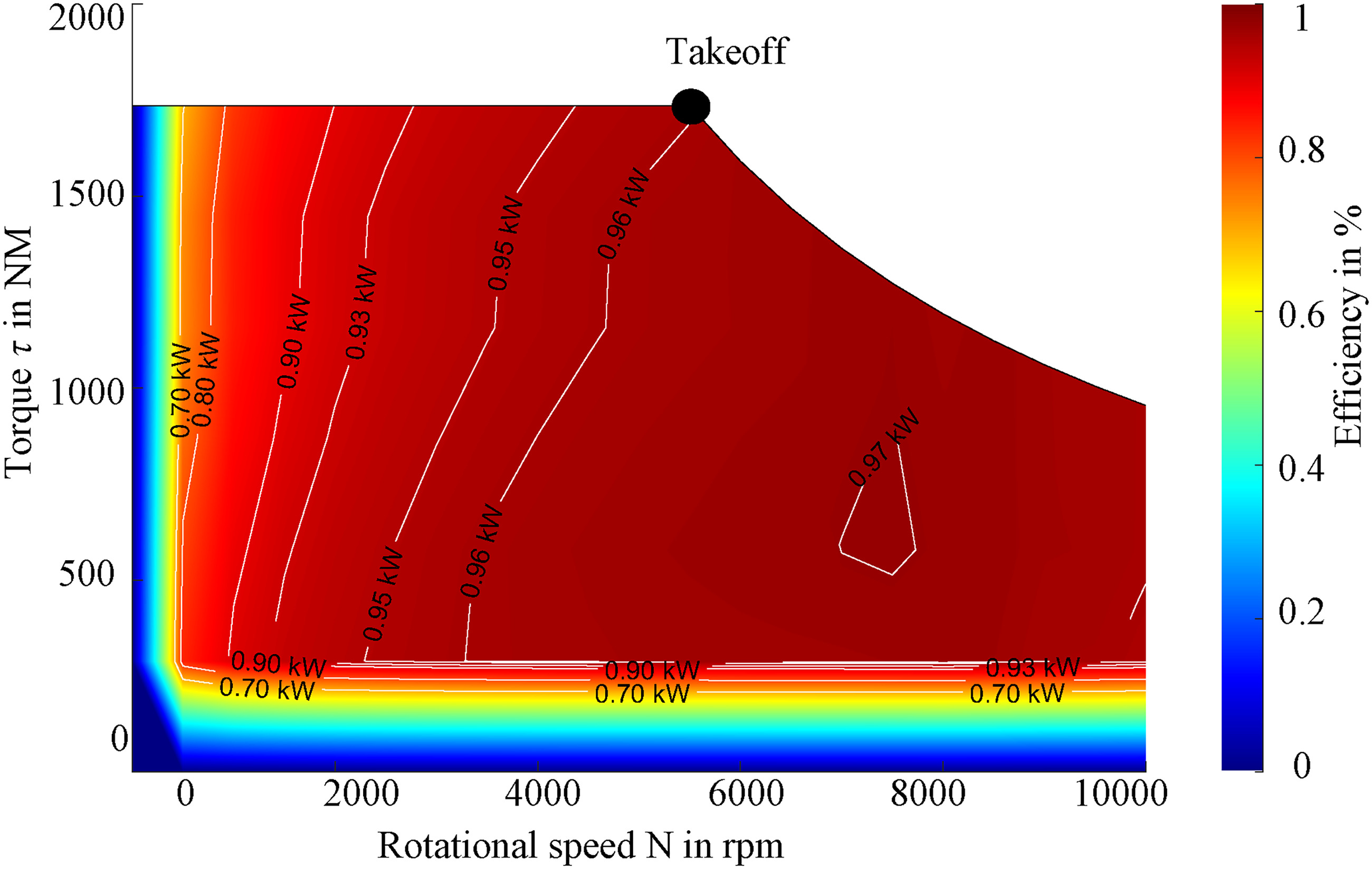
The EM designed by means of a finite element method is of a 9-phase design and has a power density of 6.86 kW/kg. The total weight of the electrical machine is 145.7 kg. The 9 phases are divided into three 3-phase systems each, which are necessary for the torque generation. The redundant design increases the reliability of the electrical machine because failures in one of the three 3-phase systems, which according to He et al. (2014) can account for up to 66% of the total faults, can be compensated for by the other two 3-phase systems. The main cause of the failures is due to increased partial discharge activity (Hanisch and Henke, 2022). The electric machine can basically be operated at all operating points within the characteristic diagram in Figure 3. In the control strategy presented here is operated at maximum torque
It should be noted that the parallel hybrid-electric architecture is a complex system and requires a multi-disciplinary approach for accurate analysis. The interaction between the conventional engine and the electric motor, as well as the PMAD system, must be considered. Furthermore, the electrical components’ impact on the engine’s performance, fuel consumption, and emissions must be evaluated. This necessitates the development of sophisticated mathematical models that can capture the system’s dynamic behaviour, as well as the aerothermal and mechanical characteristics of the various components.
Unsteady propulsion performance simulation
In general, the equations of motion are used to model the performance of aircraft engine as well as the temporal and spatial aerothermodynamic properties in the gas path and the system behaviour of the solid components. The equations of motion are divided into the continuity, momentum, and energy equations (Liepmann and Roshko, 2001). The focus of the modelling is on the overall system performance, which considers only the 1D flows in the gas path. The system of differential equations 1 describes the conversation of mass, momentum, and energy with the cross-section A, density
Due to the complexity of the equations of motion, various numerical approaches are used to solve the differential equation system. In general, the methods can be classified into stationary and unsteady models. The unsteady models can also be divided further into transient and dynamic methods. Essentially, transient effects are observed on time scales of seconds to minutes, while gas dynamics are on the order of milliseconds (Garrard, 1995). For the unsteady performance simulation, a steady-state initial point is required. Therefore, an iterative process, based on the constant-mass-flow (CMF) method is used (Kurzke and Halliwell, 2018; Goeing et al., 2023). The unsteady performance of the parallel hybrid-electric turbofan engine is simulated with a dynamic approach and the transient CMF method.
Dynamic model
Based on the governing equation system 1, an ordinary differential equation system is spatially discretised (see Equations 2–6), which represents the quasi 1D gas path and describes the dynamic approach Sugiyama et al. (1989). The component characteristics are included via the surface forces
Furthermore, the heat flux between components and gas path are characterised by the
Finally, the change in rotational speed is determined based on the applied torques of the turbines
This system was implemented in MATLAB/-Simulink 2019a. The ordinary differential equation system is solved using a variable-order method, which sets the time step with a relative tolerance of
Constant mass flow method
The transient CMF method is illustrated by the flowchart in Figure 4. Based on a steady-state operation point, a global cycle process calculation is performed. In contrast to the steady-state CMF method, an imbalance between the compressor and turbine torque is allowed (Palmer and Cheng-Zhong, 1985; Kurzke and Halliwell, 2018) to compute the change in rotational speed (see Equation 8). The iteration variables are varied until the steady state continuity equation and expansion conditions are satisfied within the time step. The momentum equation is not included. Once the steady state target functions have converged, the transient operating point is reached, and the rotational speeds for the next time step are integrated from the time-dependent power difference. The new time step is initiated by changing the fuel flow

Based on the energies in the gas path and materials, the heat fluxes and thus the temperatures are updated after each iteration (Walsh and Fletcher, 2004). Thus, the information is not fed back during one iteration and does not affect the transient cycle process. Compared to the dynamic approach, aerothermodynamic interdependencies within the gas path as well as with the entire thermodynamic cycle are not taken into account.
The performance maps of the components are used form Goeing et al. (2020) and the models are validated in Goeing et al. (2021). Although the methods access the same gas tables, performance maps and correction models, parameter errors exist due to the different solution approaches. This maximum parameter error is 0.2% (Lück et al., 2022).
For further use, the surge margin
The deviation
Results and discussion
A fuel flow signal is defined and implemented as an input signal in the transient and dynamic model to investigate the aerothermodynamic interdependencies. The manoeuvre involves slam acceleration and deceleration between 11 kN and 103 kN. The fuel flow signal is shown in Figure 5a. The conventional aircraft engine is shown in blue, connected to a 1 MW EM in green and a 2 MW EM in purple. Based on hybridisation, the aircraft engine with the 2 MW motor requires the least amount of fuel during takeoff. The fuel supply is increased between 0.1 s and 1.6 s and decreased between 6.1 s and 7.6 s (dashed line).
Figure 5.
(a) Definition of the fuel flow signal; (b) relationship between thrust F N P M

Furthermore, Figure 5b illustrates the operating strategy of the electric motor. It is switched on at 30% of the maximum thrust (using
Aerothermodynamic interdependencies
Firstly, this section explains the aerodynamic interdependencies that exist in a conventional aircraft engine. For this purpose, the CMF method is compared to the dynamic approach, with a particular focus on the HPC without hybridisation and heat flux. Figure 6a shows the predicted time-dependent operating line. The dashed blue line represents the dynamic approach, while the blue solid line shows the CMF method. The curves are presented in the HPC performance map, which depicts the black speed curves in terms of pressure ratio
Figure 6.
Numerical comparison of the HPC operating line. Left: operating line simulated by the dynamic approach and the CMF method. Right: deviation of the pressure ratio, mass flow and SM
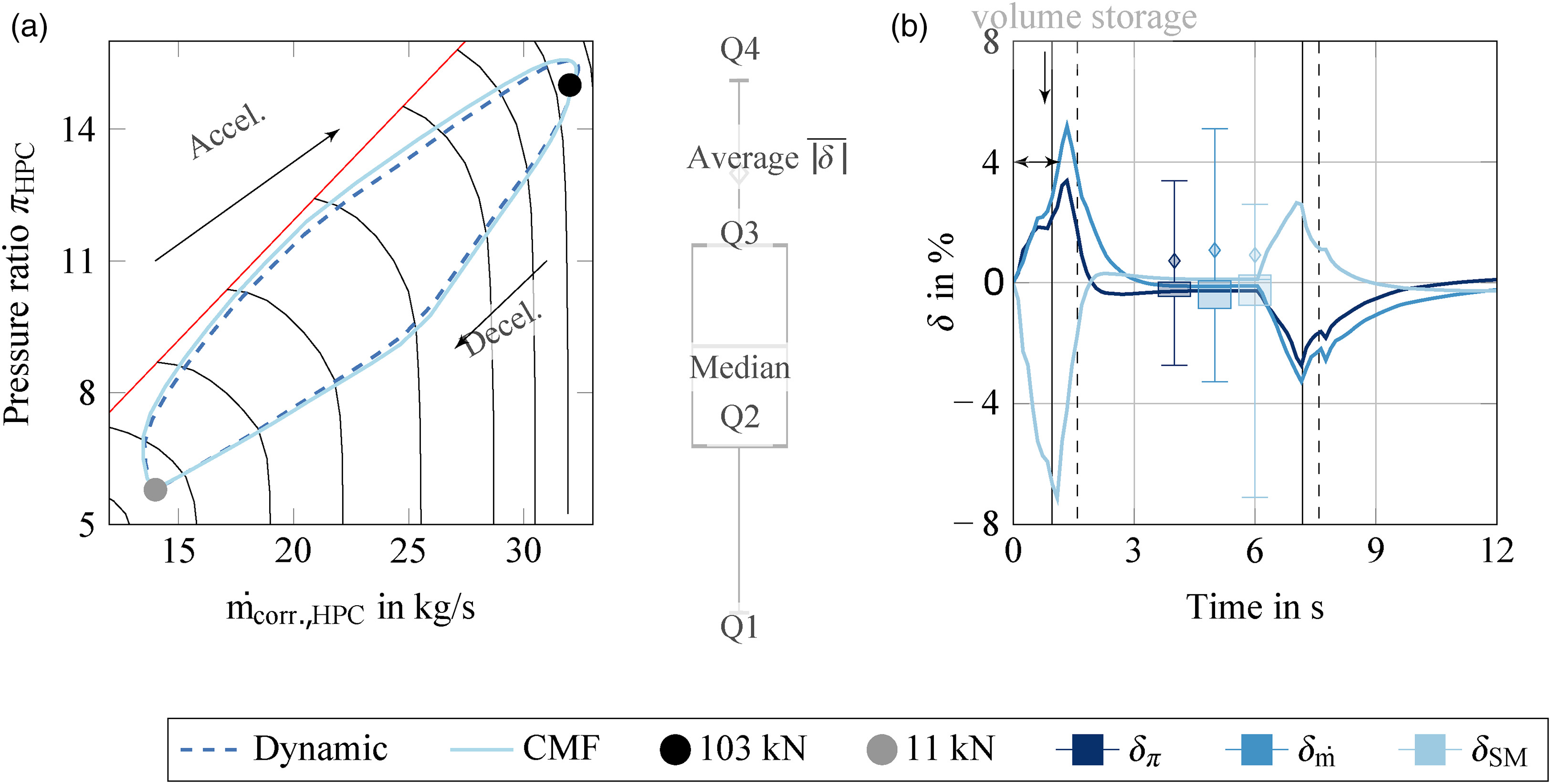
In Figure 6b the deviations
The impact of the volume storage effect on the cycle process is particularly evident in the case of the FAR, which is shown in Figure 7a for the different components over time. The profiles demonstrate that the results of the dynamic model have significantly higher FAR in the combustor (FAR4), high-pressure turbine (FAR41), and low-pressure turbine (FAR45), than the results of the CMF method. The direct influence of volume storage reduces the mass flow rate during acceleration. This reduction in mass flow rate increases the FAR. This aerothermodynamic interdependence is only captured by the dynamic model, resulting in the CMF method predicting a smaller FAR (see magnification). Furthermore, the relative deviations of FAR4, FAR41 and FAR45 of are shown in Figure 7b. As expected, the different variations of the FAR behave similarly and are significantly influenced by the core mass flow.
Figure 7.
Numerical comparison of FAR. Left: FAR simulated by the dynamic approach and the CMF method. Right: deviation of the FAR between the dynamic approach and the CMF method.

Figure 8 illustrates the process of fuel mass flow rate changes, using the example of control volumes of the turbines and the entire cycle process within one time step. Changing the fuel flow leads to a new

These aerothermodynamic interdependencies become significantly more complex due to further secondary effects. Using heat transfer as an example, this section illustrates how the heat fluxes
Heat fluxes
To advance the exploration of aerothermodynamic interdependencies, the convective heat transfer within the turbines of an aircraft engine, specifically between the gas path and materials is considered. For this purpose, the same surrogate models and correlations for discs, blades, and housings are used in the CMF method and in the dynamic model (Stephan et al., 2019; Li et al., 2022). In Figure 9a, the temperature profiles of the miscellaneous components are shown, while the box plot of relative temperature deviations is displayed in Figure 9b. The results of the deviation between the CMF and dynamic model with heat convection are illustrated in yellow and compared to the box plots from the previous subsection without heat fluxes in the same figure in blue. The temperature profiles can be qualitatively divided into temperatures upstream and downstream of the combustor. The predicted temperatures of both methods simulate qualitatively comparable profiles. The largest discrepancies are visible in

Level of hybridisation
In this section the influence of hybridisation on the aerothermodynamic interdependence is examined in this section without heat transfer. For this purpose, the operating strategy shown in Figure 5b is used and connected to the 1 MW or 2 MW motors (see Figure 3). Due to the hybridisation of the aircraft engine, the LPC represents a critical component. The performance is examined more closely in Figure 10. In Figure 10a, the unsteady operating line during the manoeuvre of the LPC can be seen. The conventional aircraft engine without an electric motor is represented in blue, with 1 MW hybridisation in green, and with 2 MW in purple. The dynamic model is shown with the dashed lines and the CMF method with the solid lines. The diagram shows that the steady-state operating points are throttled at 103 kN by hybridisation, while the operating characteristics are identical at 11 kN (here, the EM is switched off). The use of the EM during time-dependent operation changes the unsteady operating characteristics and operates closer to the stability line. In Figure 10b, the differences of the SM between the CMF and the dynamic model are displayed. The plots exhibit a qualitatively similar behaviour. However, the box plots in the middle of the diagram demonstrate that the Q1 until Q4 and the median deviations increase due to the hybridisation. It is evident that the deviations in acceleration are particularly pronounced during engagement of the EM [also visible in the magnification of diagram (a)]. The deviations increase due to the control with the
Figure 10.
Impact of hybridisation on the LPC. Left: operating line during the transient manoeuvres of different aircraft configurations. Right: deviation of the S M LPC

Finally, in Figure 11, the box plots of the deviations from the surge margin in diagram (a) as well as the thrust and rotational speeds in diagram (b) are shown. The results show the deviation with heat flux enabled for different levels of hybridisation. The deviations of the SM between the dynamic and CMF method increase in the LP-System and decrease in the HPC (see Figure 11a). This can be justified by the control strategy, as well as by the reduced stress on the HPC due to the hybridisation, which results in a smaller fuel flow step (see Figure 5). Furthermore, the diagram (a) shows that the LPC is most sensitive to the interactions and exhibits deviations of up to −13% (Q1). Also the aerothermodynamic interdependencies of the heat transfer increase the deviation significantly (compared to Figures 6 and 10).
Figure 11.
Numerical comparison between the dynamic approach and the CMF method with heat flux and different levels of hybridisation.

The influence of the control strategy on the deviation is also visible in diagram (b). While the deviations of
Conclusions
In this study, the influence of aerothermodynamic interdependencies on the unsteady system performance of a hybrid-electric turbofan is investigated. Aerothermodynamic interdependencies refer to the interaction between unsteady effects, such as volume storage or heat transfer, in a time-dependent manoeuvre. Initially, the aerothermodynamic interdependencies are illustrated using a conventional turbofan engine as an example, by simulating the performance during a slam acceleration and deceleration with a dynamic approach and the constant mass flow (CMF) method. In this case, only the dynamic approach is able to model the aerothermodynamic interdependencies, while the CMF method uses steady-state conditions in the gas path. Next, heat transfer in the hot gas path is considered to increase the number of secondary effects. Finally, the system complexity is increased by the level of hybridisation with a 1 MW or 2 MW electric motor, which is engaged during the manoeuvre to support the fan at its maximum thrust. The results of the comparison can be summarised as follows:
The volume storage effects lead to an interdependence between mass flow and fuel to air ratio, which affects the entire joule process.
Additional secondary effects such as heat transfer can reduce the maximum discrepancies but increase the average deviations in the entire joule cycle process, especially in the low-pressure compressor (LPC).
Hybridisation increases the load of the LPC and decreases the load of the high-pressure compressor (HPC).
Interdependence due to the hybridisation increases the deviation of the LPC between the dynamic approach and the CMF method.
Nomenclature
Efficiency
Pressure ratio
Mass flow
Fuel flow
bleed flow
Heat transfer coefficient
Torque
Institute of jet propulsion and turbomachinery
Institute for electrical machines, traction and drives
Exhaust gas temperature
Heat flux
Temperature
Total
Time
Pressure
Bypass ratio
Rotational speed of LP-system
Rotational speed of HP-system
Constant mass flow
Specific fuel composition
Thrust
High-pressure compressor
High-pressure turbine
Low-pressure turbine
High-pressure system
Low-pressure system
Low-pressure compressor
Enthalpy
Surge margin
Surge line
Wall temperature
Fuel to air ratio
Operating point
Surface
Density
Volume
Area
Darcy friction
Surface forces
Diameter
E-Motor
Moment of inertia
Length
Deviation
Velocity
Internal energy