Introduction

Three-dimensional computational fluids dynamics (CFD) is critical to compressor and fan stage blade design and assessment, and for accurate determination of stall margin, most commonly unsteady Reynolds-averaged Navier-Stokes (URANS) computations are used. In the industrial design cycle, though, URANS can still be prohibitively expensive. There is thus a strong motivation to gain confidence in turbulence modelling approaches which enable accurate stall point determination with steady RANS. This requires accurate determination of the onset of flow separations. In particular, it is critical that corner separations are accurately captured.

Menter’s shear stress transport (SST) model (Menter, 1994), the Spalart-Allmaras (SA) model (Spalart and Allmaras, 1992) and modifications of these are widely used in turbomachinery. The SST model has proved to accurately predict secondary flows near corners in RANS (Menter, 2009). Yin et al. (2010) carried out computations for an axial compressor using both the SST and SA models. They compared the compressor’s mass flow rate at choke for the design speed, and it was found that the SST model matched the experimental data to within 0.344% while the SA model over-predicted the choking mass flow rate by 6.6%. Notably, although the computed results with the SST model were accurate overall, the tip clearance/shock interaction loss was underestimated, so there is room for improvement.

To predict compressor and fan behaviour more accurately, Liu et al. (2011) modified the original SA model by introducing the helicity to take the turbulence energy backscatter into consideration. Following Liu et al.’s idea, Lee et al. (2018) introduced the helicity correction to the SA model and added the effects of adverse pressure gradients, applying the updated model to a fan simulation. This method increased the turbulent viscosity in the region of shock wave boundary layer interactions, which directly improved the accuracy of separation point prediction and consequently showed the CFD choking mass flow at 100% speed was only 0.6% above the measured value. Kim et al. (2019) investigated rotating stall in a transonic fan by adopting the modified SA model from Liu et al., and they found that the modified SA model predicted the stall inception mechanism to be consistent with the experimental data. Notably, both RANS and URANS computations with the modified SA model were conducted in Kim et al.’s work, and RANS was able to accurately predict the fan performance characteristic, in line with URANS and experiments. Both papers showed that it was possible to accurately predict the stall point at low computational cost by using the modified SA model in compressible flow. However, since their modifications focused on capturing shock-boundary layer interactions, for lower Mach number flows without strong shocks it is not clear if their modified model is appropriate. In Liu et al.’s research (Liu et al., 2011), their modified SA model was originally assessed for incompressible flow in a linear cascade, and the modified turbulence model was shown to predict the corner separation much more accurately than the original SA model. This approach is known as the helicity-corrected SA (HCSA) model. Lopez et al. (2022) performed steady compressible flow simulations using the HCSA model to reveal the effect of tip leakage axial-momentum flux on design point efficiency and stability range for a transonic axial fan, and they were able to predict stalling mass flows to within 0.81% and 3.8% of experimental data for a reference design at 103% and 95% speeds, respectively. Yu et al. (2023) implemented the HCSA model in OpenFOAM v2206 (ESI, 2022) and applied it to stall prediction for a single-stage axial fan with incompressible flow, finding that the stall margins predicted with the HCSA model in steady RANS and URANS were predicted to within 1.2% and 0.2% of design flow coefficient, respectively.

The backward energy transport, termed energy backscatter by Leith (1990), exists in all kinds of turbulence. In the theory of Lesieur (2008), energy backscatter is evident in regions with coherent structures like mixing layers and rotating turbulence. A lack of backscatter can lead to inaccurate flow field predictions for the internal flow in compressor and fan blade passages. Liu et al. (2011) found that the helicity is able to represent the energy backscatter, and so they modified the SA model by introducing the helicity into the production term of the SA variable transport equation. They assessed the modified model’s ability to predict corner separation in a linear compressor cascade by comparison to experimental data, showing that the HCSA model accurately determined the location and size of the corner separation.

The SA model is a one-equation (Spalart and Allmaras, 1992) model that solves the transport equation for the modified kinematic turbulence viscosity ν~, and the kinematic turbulence viscosity νt is calculated by

where the function fv1 is

In Equation 2, the constant Cv1=7.1 and

where ν is the molecular kinematic viscosity.

The transport equation for ν~ in the original SA model is

where D/Dt denotes the substantial derivative and

In Equations 4–9, ω¯ is the vorticity, ρ is the fluid density, d is the distance from the wall, and Cb1, Cb2, Cw1, Cw2, Cw3, σν~, and κ are constants whose values can all be found in Spalart and Allmaras’ original paper (Spalart and Allmaras, 1992).

In the HCSA model, the coefficient of the vorticity term in S~ (Equation 8) is modified to depend on the normalized helicity. The modified S~MSA, which replaces S~, is

where Ch1 is 0.71 and Ch2 is 0.6, according to Liu’s numerical tests. The normalized helicity h is

where v is the velocity.

The HCSA model computation in Liu’s research was carried out in Ansys FLUENT (Ansys Inc., 2023) and the implementation’s source code is not available. In addition, the linear cascade used as a validation case by Liu et al. is based on geometry that is not publicly available.

The aims of this paper are to (1) demonstrate the implementation of the HCSA model in an open-source code, and (2) gain insight into the underlying differences between the SA, HCSA, and SST turbulence models which cause differences in predicted flow separation behaviour in compressor blade passages. Since Liu et al. (2011) implemented the HCSA model and tested its ability of flow separation predicting on a linear Prescribed Velocity Distribution (PVD) cascade, in this paper, we instead work with a NACA 65-1810 linear cascade. Steady-state incompressible flow simulations for the SA, HCSA, and SST models are carried out to compare the accuracy of flow separation prediction relative to experimental data, and to gain insight into how the manner in which the turbulence models are formulated affects that accuracy.

The remainder of this paper is organized as follows. First, we introduce the linear cascade used as a test case. In the methodology section, the grid details, and the computational approach with OpenFOAM is introduced. The results and discussion section focuses on the comparison of the three different turbulence models with experimental results, as well as analysis to explain the improvements seen with the HCSA model.

Test case

The case studied is from Kang and Hirsch’s (1991) experiment. They investigated a low-speed linear compressor cascade in a blower-style configuration wind tunnel. While data is only available at design incidence, Liu et al.’s results (Liu et al., 2011) for a different cascade shows similar performance for the SA and HCSA models to what will be shown in this paper, suggesting that the findings are applicable to a variety of blade designs and loading distributions.

Returning to Kang and Hirsch’s experiment, the inflow passes through a row of guide vanes, a diffuser, a setting chamber, and a nozzle before reaching the test section. The test section consists of 7 blades, installed between two parallel plates which were aligned horizontally. A 3 cm gap is introduced between the two extreme blades and the nozzle side wall to remove the side wall boundary layers. There are two variable flaps placed at the exit of the two extreme blades to maximize the periodicity for the central blades.

Methodology

In this section, we introduce the computational details used in this paper for studying the turbulence models.

Grid generation

AutoCAD version 2023 (Autodesk Inc., 2022) is used to generate the cascade blade geometry from the NACA 65-1810 blade coordinates in (Kang and Hirsch, 1991). The computational domain, spanning a single blade passage, is generated using the OpenFOAM tools blockMesh and snappyHexMesh. The domain is initially created without the blade present using blockMesh, and then the blade shape is subtracted, and the surrounding grid refined using snappyHexMesh. Boundary layers cells are added on the blade surface by snappyHexMesh and the OpenFOAM tool refineWallLayer is used successively to create the endwall boundary layer cells. Figure 1a shows the blade-to-blade view of the cascade mesh. The inlet and outlet boundaries are located 40% and 150% of the blade chord away from the blade leading and trailing edges, respectively. The inlet is close to the leading edge, but this location is used since the inlet conditions (including endwall boundary layer details) are specified in Kang and Hirsch’s paper (Kang and Hirsch, 1991) at this location. The computational domain covers half the span, with a symmetry plane specified at mid-span, since the inlet condition is symmetric, and Kang and Hirsch’s results focus on the flow details near the upper endwall. Cyclic (periodic) boundary conditions are used to enable use of a single passage domain. 17 boundary layer cells are used with a first cell target y+ of 3 on both the endwall and blade surfaces. Figure 1b shows both boundary layer grids where the endwall and blade suction surface meet.

Figure 1.

Linear cascade mesh: (a) blade-to-blade view and (b) detail of the boundary layer cells where the endwall and blade suction surface meet.

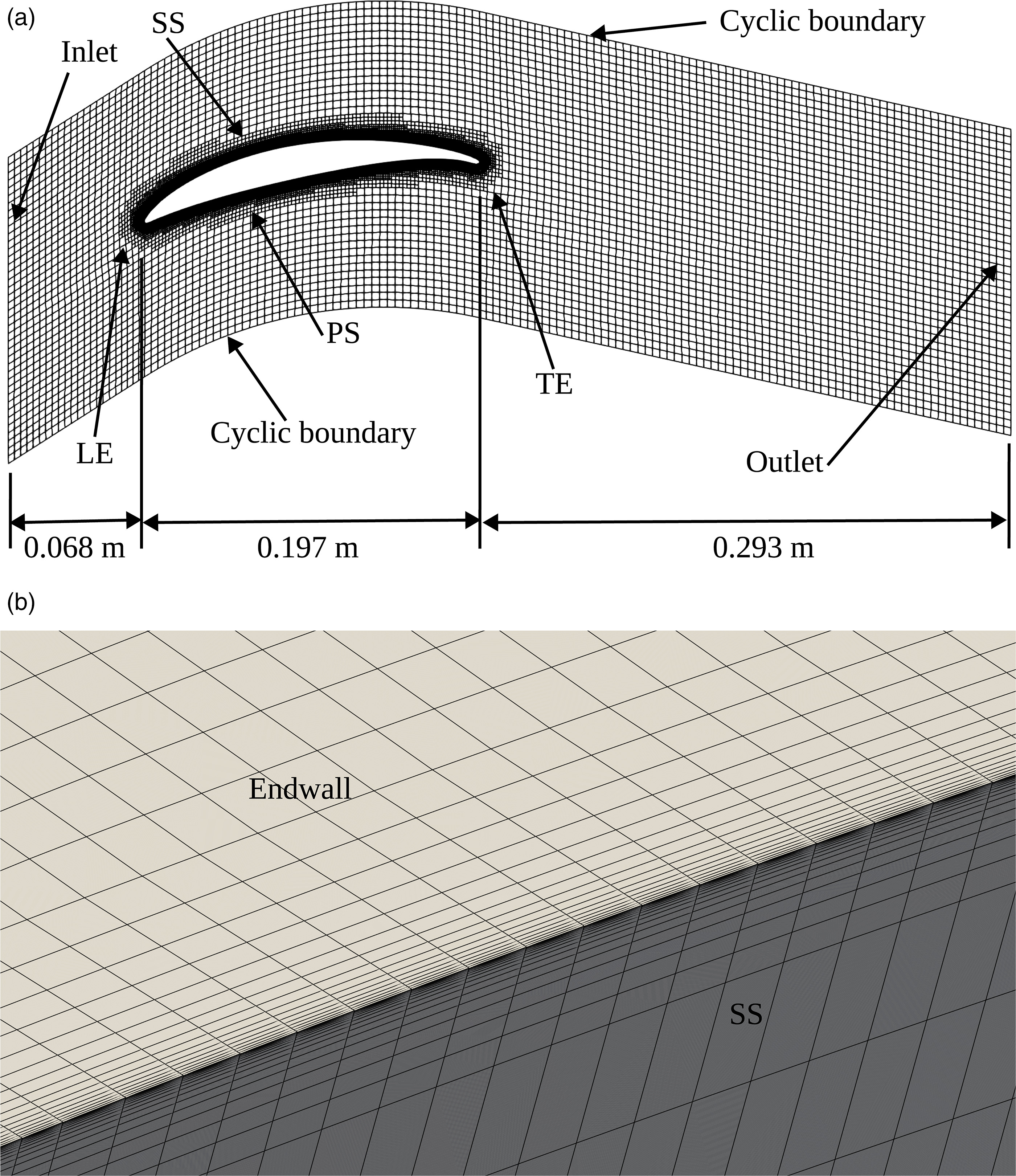
The overall cell count is approximately 2.9 million cells. To establish grid independence, grids with 0.6 million, 1 million, 1.64 million, and 3.3 million cells were also assessed. The mass-averaged total pressure loss between the inlet and outlet increased by 1.18% between the 2.9 million and 3.3 million cell grids. Compared with the averaged total pressure loss change at 12% among the 0.6 million, 1 million, and 1.64 million grids, the 2.9 million cell grid was suitable for all computations in this paper. Additional details on the grid independence assessment can be found in Yu et al. (2023).

Results and discussion

All computations are performed at the design incidence (−2.5∘). The computed and experimental blade surface static pressure coefficient Cp distributions at 99%, 98.5%, and 50% span are shown in Figure 2. Cp is defined as:

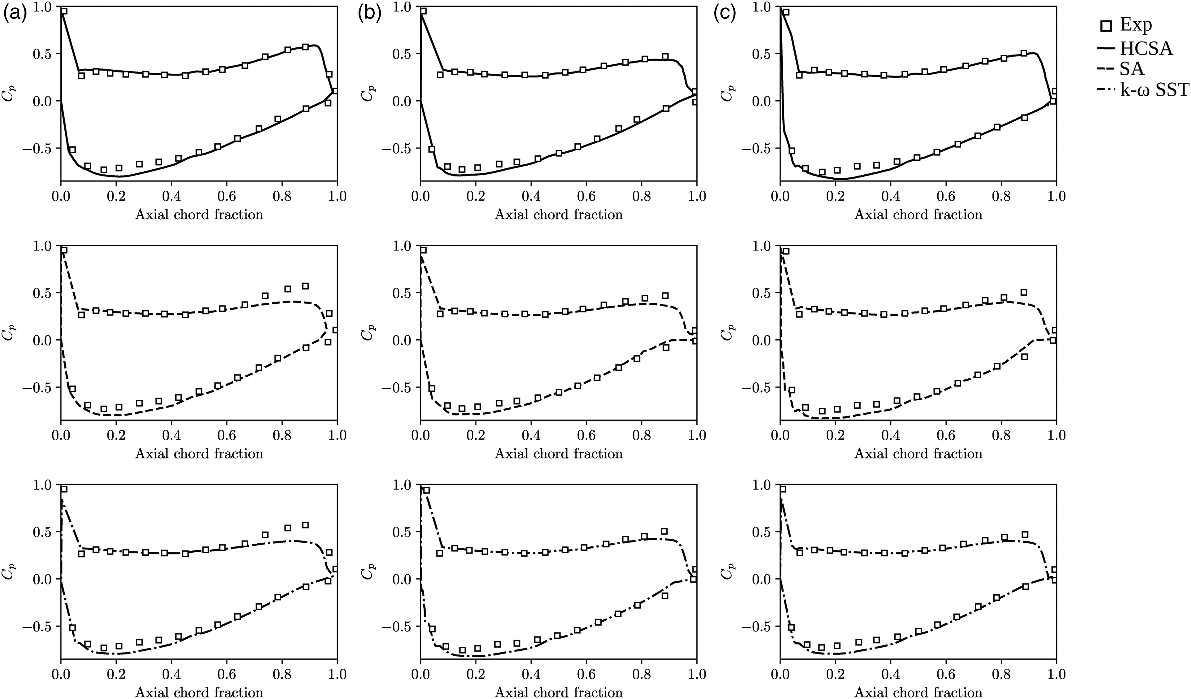
Figure 2.

Surface static pressure coefficient at (a) 99% (b) 98.5% (c) 50% span for the cascade at design incidence. Open squares: experimental data (Kang and Hirsch, 1991); solid line: CFD with HCSA turbulence model; dashed line: CFD with SA turbulence model; dash-dotted line: CFD with k−ω SST turbulence model.

where p1 and p are the inlet and local static pressures, respectively.

From Figure 2, the HCSA model accurately predicts the blade loading across the span. At 98.5% and especially at 99% span, the corner separation size is over-estimated by the SA and SST models, but the HCSA correctly predicts that the flow remains attached on the pressure surface. This improvement in the ability to capture corner separation when it physically occurs, but not to predict that it will occur when it should not, seems to be the cornerstone of the HCSA model’s benefit. This result validates the HCSA model implementation in OpenFOAM.

Turning attention to the 50% span results, the SST model is able to accurately capture the loading, as the lower loading towards the trailing edge here compared to near the endwall does not lead to over-prediction of separation. Even at midspan, the original SA model struggles to get the loading right at the trailing edge, especially on the pressure surface.

To link the changes in loading predicted by the various models to changes in loss, in Figure 3 we show the loss coefficient across the passage 25% chord downstream of the trailing edge. The total pressure loss coefficient Yp is defined as

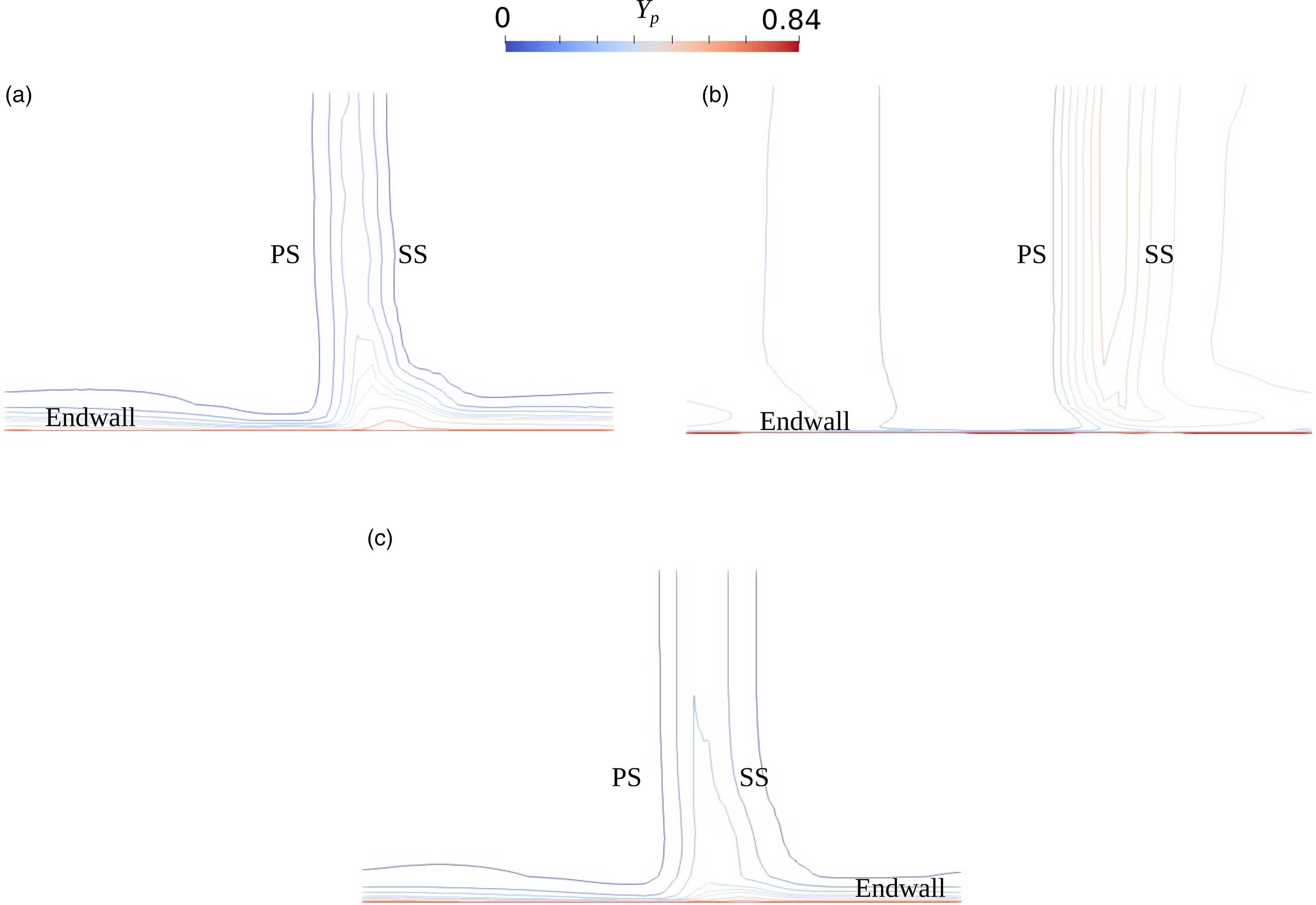
Figure 3.

Contours of total pressure losses at 25% chord downstream of the trailing edge. (a) CFD with HCSA turbulence model, (b) CFD with SA turbulence model, and (c) CFD with k−ω SST turbulence model.

where p01 is the inlet total pressure and p02 is the local total pressure on a plane 25% chord downstream of the trailing edge.

The HCSA model results are in good agreement with the experimental results reported by Kang and Hirsch; the detailed experimentally measured total pressure losses can be found in Figure 9 of their paper (Kang and Hirsch, 1991).

The loss coefficient contours enable visualization of the size, intensity, and location of the corner separation. The corner separation size is overestimated by the SA model compared with the HCSA model, and instead of a concentrated region of high loss close to the endwall, the high loss region persists up the span – there is much less three-dimensional structure to the loss contours for the SA model. Comparing these two models’ results in more detail, the level of loss predicted by the SA model rises moving away from the endwall, while for the HCSA model the high loss region is confined to the outer span. This explains why the static pressure coefficient is lower than the measured values at all spans in Figure 2 for the original SA model. Figure 3c demonstrates that the SST model results are somewhat of a middle ground: the predicted corner separation size is larger than it should be near the endwall, but the loss level decreases moving towards midspan. This is consistent with the increased level of accuracy for the SST model at midspan in Figure 2 compared to near the endwall.

To determine why the loss coefficient distributions are so different for the three turbulence models, Figure 4 depicts the normalized kinematic turbulent viscosity distribution νt/ν at the same location as in Figure 3. The most significant difference between the three models is that only the HCSA model captures the concentrated region of high turbulent viscosity associated with the corner (shed) vortex, which was also seen by Kang and Hirsch (1991). The shed vortex located near mid-span, also at a similar spanwise location as observed in the experiment, is a vortex that is neither the trailing shed vortex nor the trailing filament vortex. The specific reason for this concentrated shed vortex is not clear, but Kang and Hirsch speculated it originates from the spiral node point generated by the separation lines on the suction surface. Although the detailed cause of the shed vortex at mid-span requires further investigation, the HCSA model is able to accurately capture both these regions of high vorticity and turbulent viscosity.

Figure 4.

Contours of normalized kinematic turbulent viscosity from the endwall to mid-span at 25% chord downstream of the trailing edge. (a) CFD with HCSA turbulence model, (b) CFD with SA turbulence model, and (c) CFD with k−ω SST turbulence model.

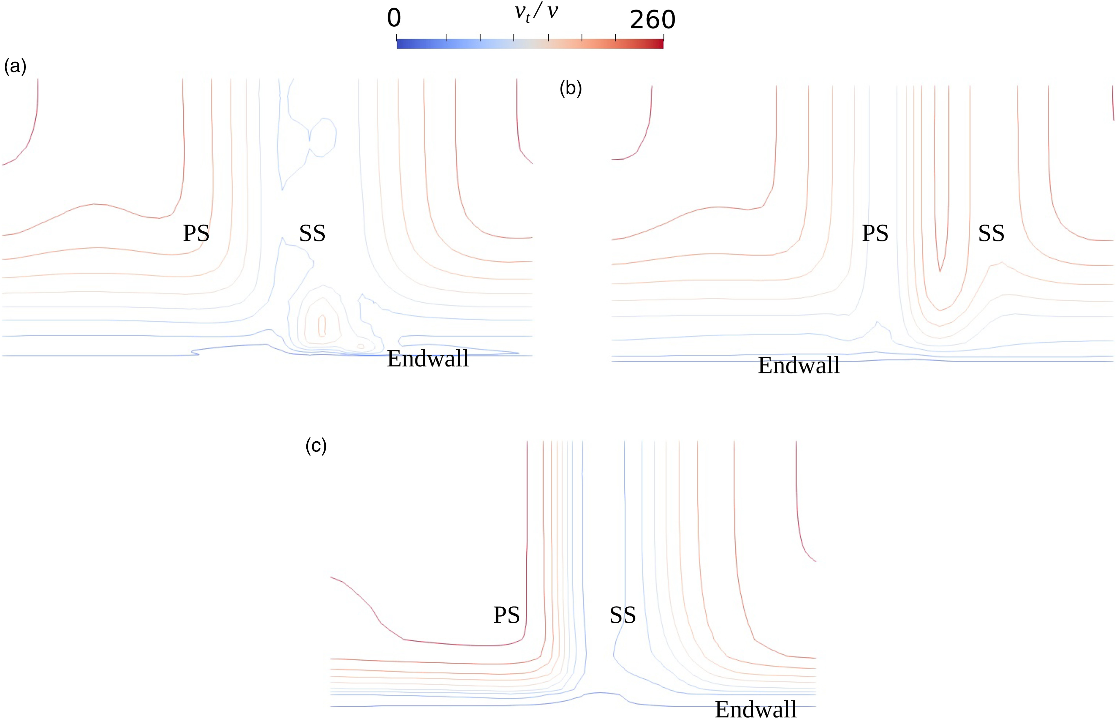
The turbulent viscosity contours also indicate that the SA model predicts the corner separation to be too large and to persist up the span (Figure 4a). The SST model fails to show a distinct vortex core in the turbulent viscosity distribution (Figure 4c), though further from the endwall the distribution is more in line with the HCSA results. We next explore the reasons for the inaccurate predictions by the SA and SST models.

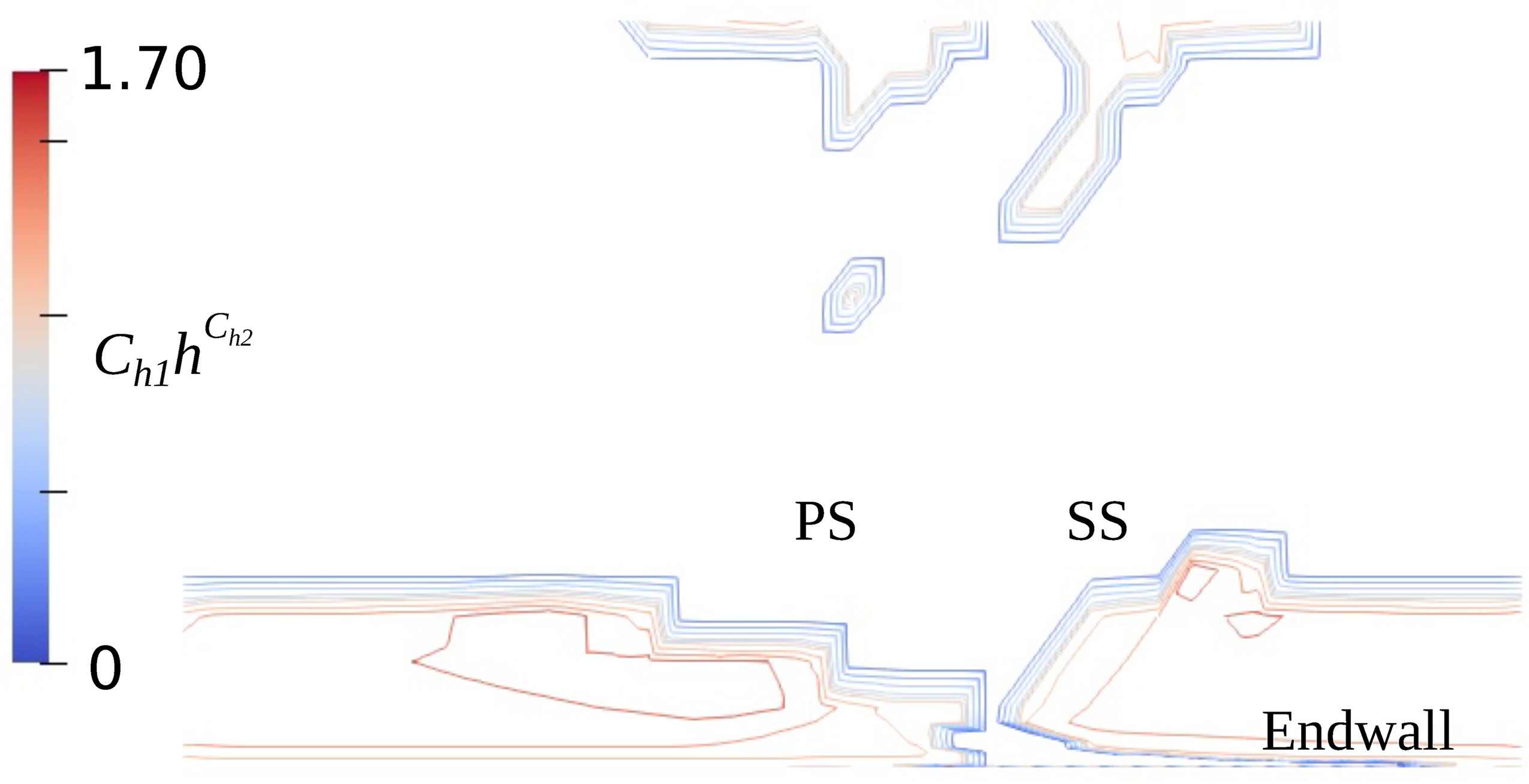
From Equations 4, 8, and 10, the modifications in the HCSA model compared with the SA model are in the production and dissipation terms of the transport equation, but an investigation of both terms indicates that the production term is the one which looks the most different between the two models. Figures 5(a) and 5(b) demonstrate the difference of production term between these two models. By introducing the corrected helicity term, shown in Figure 6, the production term in the HCSA model is able to produce additional turbulent viscosity which aids in keeping the flow attached near the endwall, preventing over-prediction of the corner separation. The helicity correction is significant (compared to 1, the term without correction) in the regions of high production near the endwall.

Figure 5.

Contours of production term in the (a) HCSA turbulence model and (b) original SA model from the endwall to mid-span at 25% chord downstream of the trailing edge.

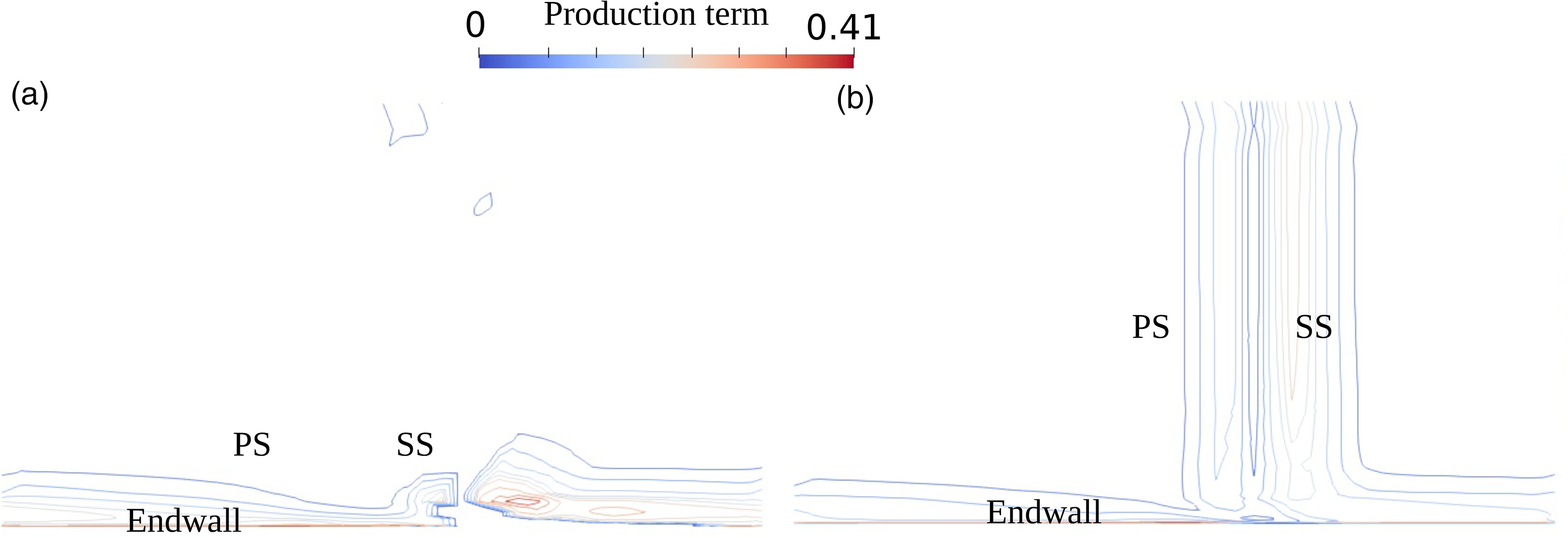
Figure 6.

Helicity correction term in the HCSA turbulence model from the endwall to mid-span at 25% chord downstream of the trailing edge.

The SST model’s calculated specific dissipation rate ω and turbulence kinetic energy k are shown in Figure 7. For the k−ω SST model, the kinematic turbulent viscosity νt is calculated as Menter (1993)

Figure 7.

k−ω SST turbulence model calculated contours of (a) specific dissipation rate and (b) turbulence kinetic energy from the endwall to mid-span at 25% chord downstream of the trailing edge.

The corner vortex is visible in the contours of turbulence kinetic energy, while the specific dissipation rate is distributed nearly uniformly along the span. The spanwise behaviour is thus dominated by k, and it can be seen that while some kind of corner vortex appears to have arisen, leading to reasonable accuracy at 98.5% span in Figure 2, it is located too far away from the endwall, so that the loading at 99% span in Figure 2 is much less accurate. Approaching midspan, the SST model predicts little spanwise variation, and is able to capture the loading correctly. The transport of k thus appears to be responsible for the misplacement of the corner vortex and thus poor prediction of the nature of the corner separation. The more complex model is still not able to capture the interaction between streamwise vorticity and loss generation, while the HCSA model is able to capture this key aspect of the flow in turbomachines.

Conclusions

In this paper, the HCSA turbulence model from Liu et al. (2011) is shown to be correctly implemented in OpenFOAM by validation using a NACA 65-1810 linear cascade for which experimental measurements are available (Kang and Hirsch, 1991). By comparing the HCSA flow field and turbulence model terms with those of the SA and SST models, some insight into the underlying reasons for the ability of the HCSA model to avoid over-predicting corner separation size is obtained. The SA model is unable to link the local helicity to the turbulent viscosity production, which leads to premature flow separation. The SST model generally is accurate away from the endwalls, but it also struggles to capture the impact of rotational flow near the endwall, resulting in the corner vortex being too large and causing separation which it should not. These findings support the advantages of the HCSA model for correctly capturing corner flow details in steady RANS computations. By using the swirling flow to produce additional turbulent viscosity, the HCSA model can avoid triggering artificial breakdown of the flow near the endwall in fans and compressors, and this is why it is able to capture the stall point with reasonable accuracy even in steady computations as has been shown by Lopez et al. (2022) and Yu et al. (2023).

Nomenclature