Investigated model

The design of rotor blade was based on the rotor blade of TTM-Stage (Erhard, 2000). Significant changes to the rotor blade of TTM-Stage were performed in order to achieve the high loading coefficient. The key geometry parameters of the blade in the cascade with the loading coefficient of 2.0 are listed in Table 1. The other blades with smaller loading coefficients were obtained by modifying turning angle based on the blade with the loading coefficient of 2.0.

Numerical method

For DDES, the SA-DDES model was employed to deal with the turbulent flow in time-dependent Navier-Stokes equations using the solver embedded into NUMECA software package. The DDES model provided additional shielding functions to ensure that the model does not switch to Large Eddy Simulation (LES) within the boundary layer in order to avoid the limitation of high sensitivity to grid spacing. The dual time stepping approach proposed was employed. At each physical time step, a steady-state problem was solved in a pseudo time. In order to speed up the convergence, the multigrid strategy and the implicit residual smoothing method were applied.

Boundary condition

The total pressure, the total temperature and the velocity vector on the inlet boundary were specified. The Mach number was obtained by extrapolation from the interior field. At the outlet boundary, the static pressure was specified. The remaining dependent variables at the outlet boundary were obtained from the interior field through the extrapolation with the zero-order.

Computational mesh

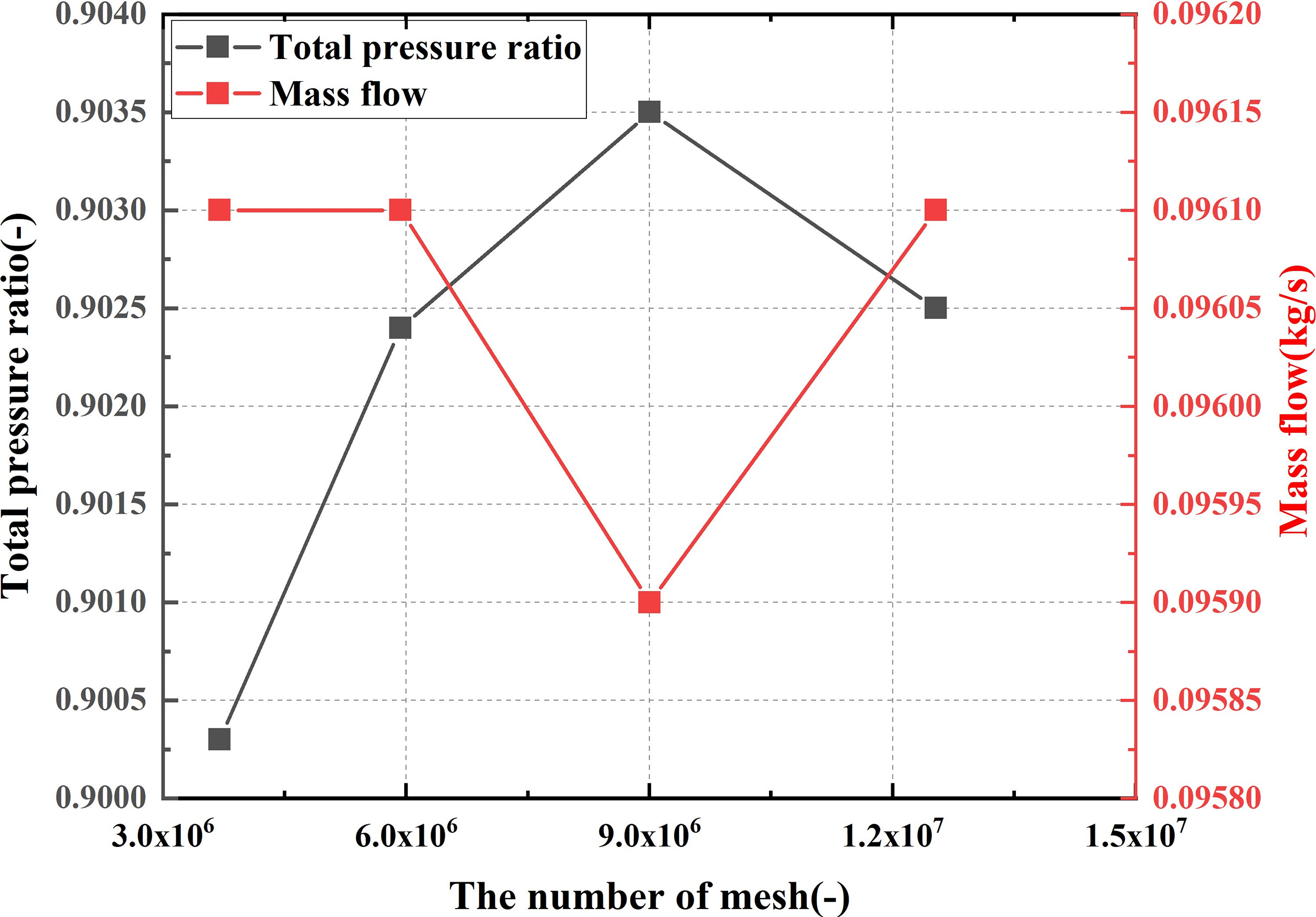
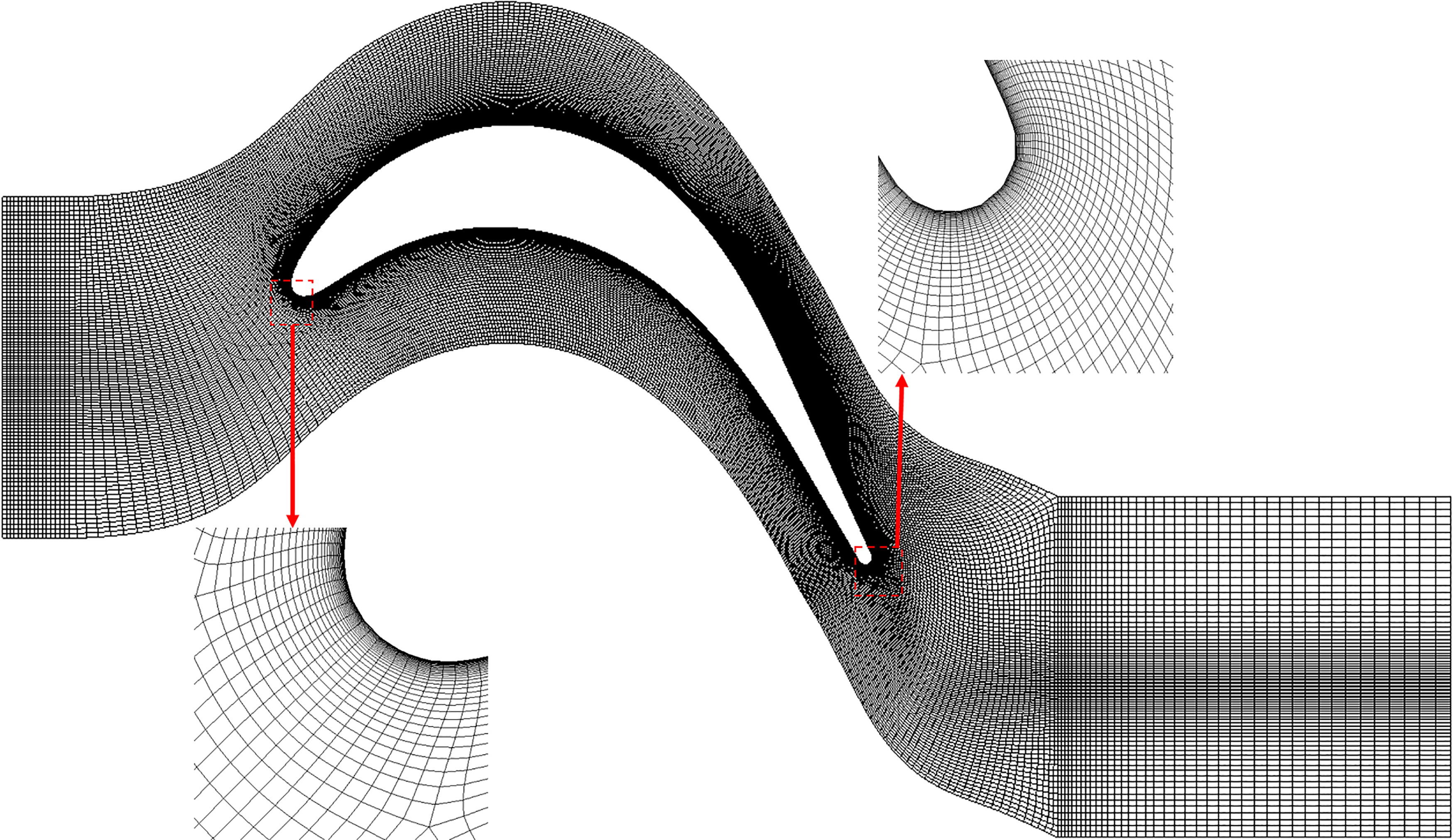
The grid was generated by the Autogrid5 module of the NUMECA software. The grid independence study was performed to confirm the reliability of the numerical simulation and the Grid independence results is shown in Figure 1. The total pressure ratio represented the ratio of the outlet total pressure to inlet total pressure. The number of 9 million grids was determined for calculation based on calculation accuracy and calculation time. Figure 2 shows the grids of the blade in cascade. The first layer grid scale was 5 × 10⁻⁶ m and the average y+ value was about 1. The physical time step was set to 1 × 10⁻⁶ s.

Figure 1.

Grid independence results.

Figure 2.

B2B computational mesh.

Convergence

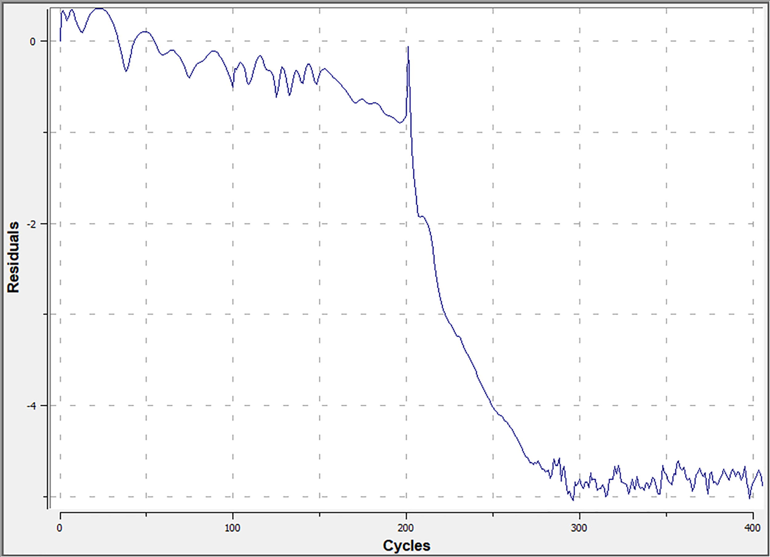
The steady calculation was carried out with 400 iterations and the DDES calculation was carried out with 350 iterations to ensure the convergence of the results. The initial condition of the DDES calculation was based on the result of the steady calculation. Figure 3 shows the root mean square global residual of the density of the RANS calculation reached 10⁻⁵ at the exit isentropic Mach number of 0.9 and the incidence angle of 0 for the blade with the loading coefficient of 2.0. The definition of the residual was the sum of the fluxes on all the faces of each cell and the data shown in Figure 3 was the logarithm of the root mean square global residual. The convergence of other conditions was similar with the convergence shown in Figure 3. The highest error in inlet mass flow and outlet mass flow was less than 0.05% and the global residual was more than 10⁻⁵ for the DDES results of all conditions.

Figure 3.

The global residual of the RANS calculation at the exit isentropic Mach number of 0.9 and the incidence angle of 0 for the blade with the loading coefficient of 2.0.

Comparison of flow fields with different exit isentropic Mach numbers

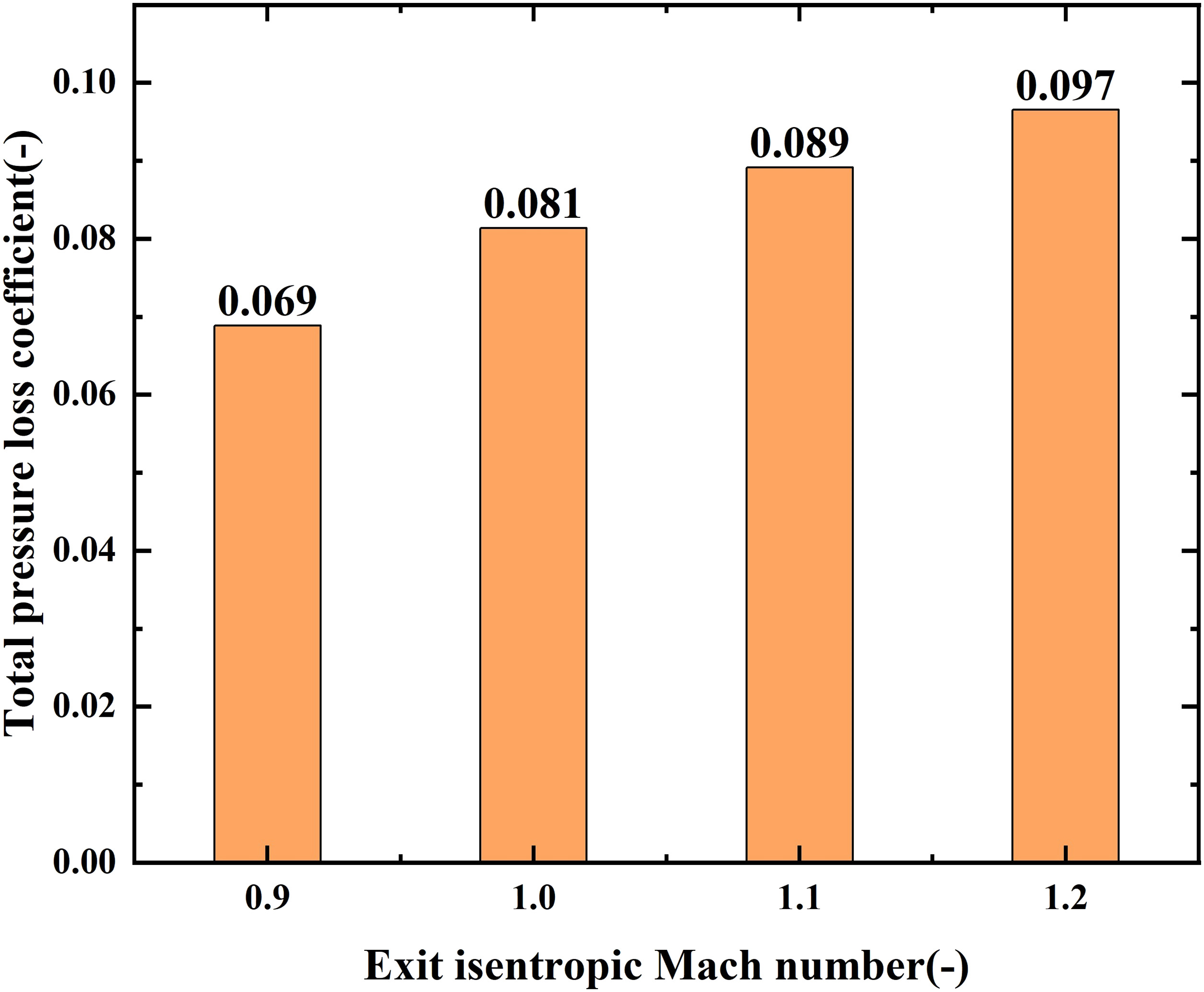
Figure 4 shows the total pressure loss coefficient at exit at loading coefficient of 2.0 and incidence angle of 0° with different exit isentropic Mach numbers. The total pressure loss coefficient is expressed by Equation 1.

Figure 4.

Total pressure loss coefficient at exit with different exit isentropic Mach numbers.

where P0∗ is the inlet total pressure, P∗ is the local total pressure.

The exit isentropic Mach number is expressed by Equation 2.

where P0freestream is the total pressure in the freestream outside of the boundary layers, usually the inlet total pressure is used, P1 is the exit static pressure and γ is the ratio of specific heat, which is 1.4 for air. When the exit static pressure is determined, the exit isentropic Mach number is changed by changing the inlet total pressure.

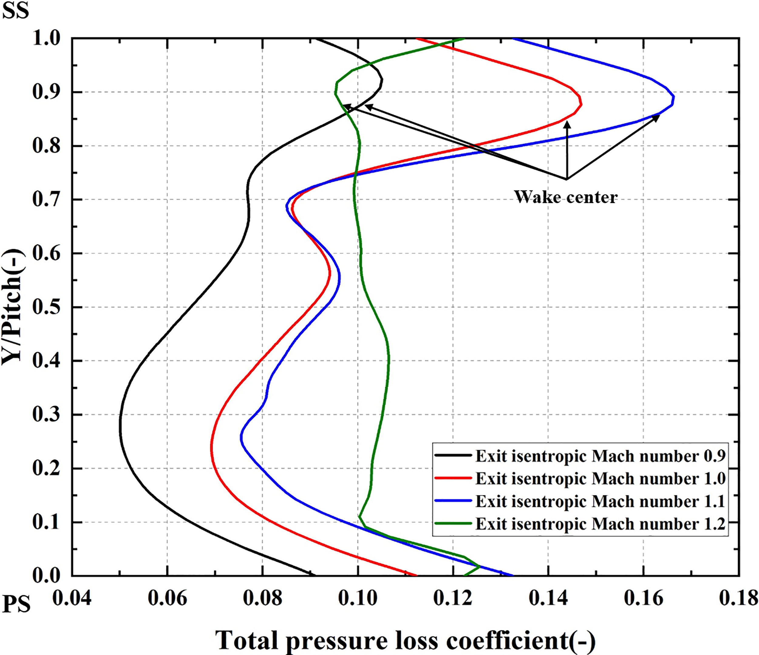
As Figure 4 shown, the total pressure loss coefficient increases with the increase of exit isentropic Mach number because of the higher Mach number and the formation of the shock wave. Figure 5 shows the total pressure loss coefficient along pitch at exit of mid-span with different exit isentropic Mach numbers. The total pressure loss coefficient shows the similar distribution when the exit isentropic Mach number increases from 0.9 to 1.1. There is a high loss region at 0.87 pitch corresponding to the wake where the loss rises from 0.105 to 0.166. At the exit isentropic Mach number of 1.2, the distribution of the total pressure loss coefficient is different from others, which is basically uniform along the pitch indicating the main flow and the wake are strongly blended.

Figure 5.

Total pressure loss coefficient along pitch at exit of mid-span with different exit isentropic Mach numbers.

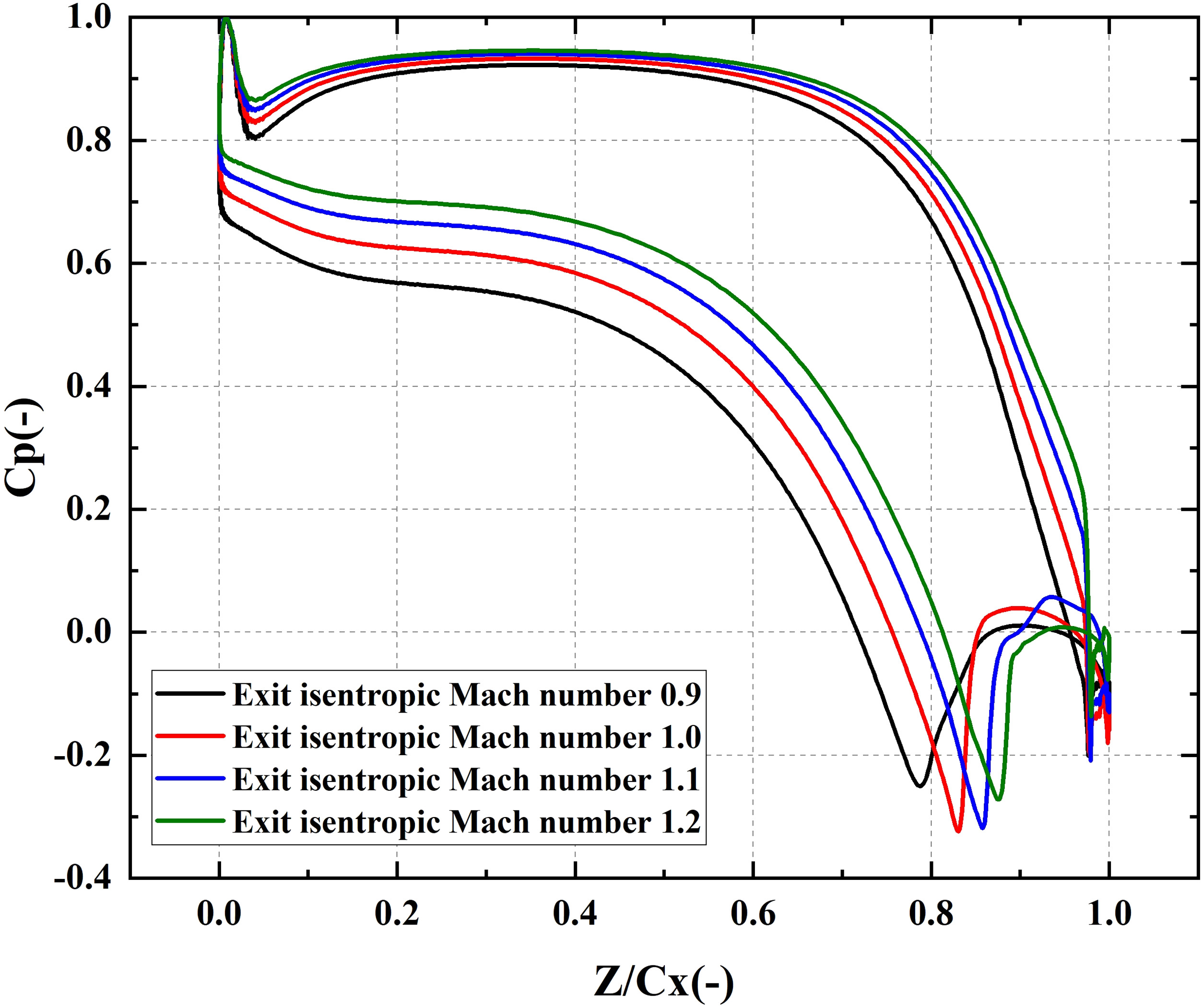
Figures 6 and 7 show the distribution of Mach number and pressure coefficient at mid-span (Cp). The pressure coefficient is expressed by Equation 3.

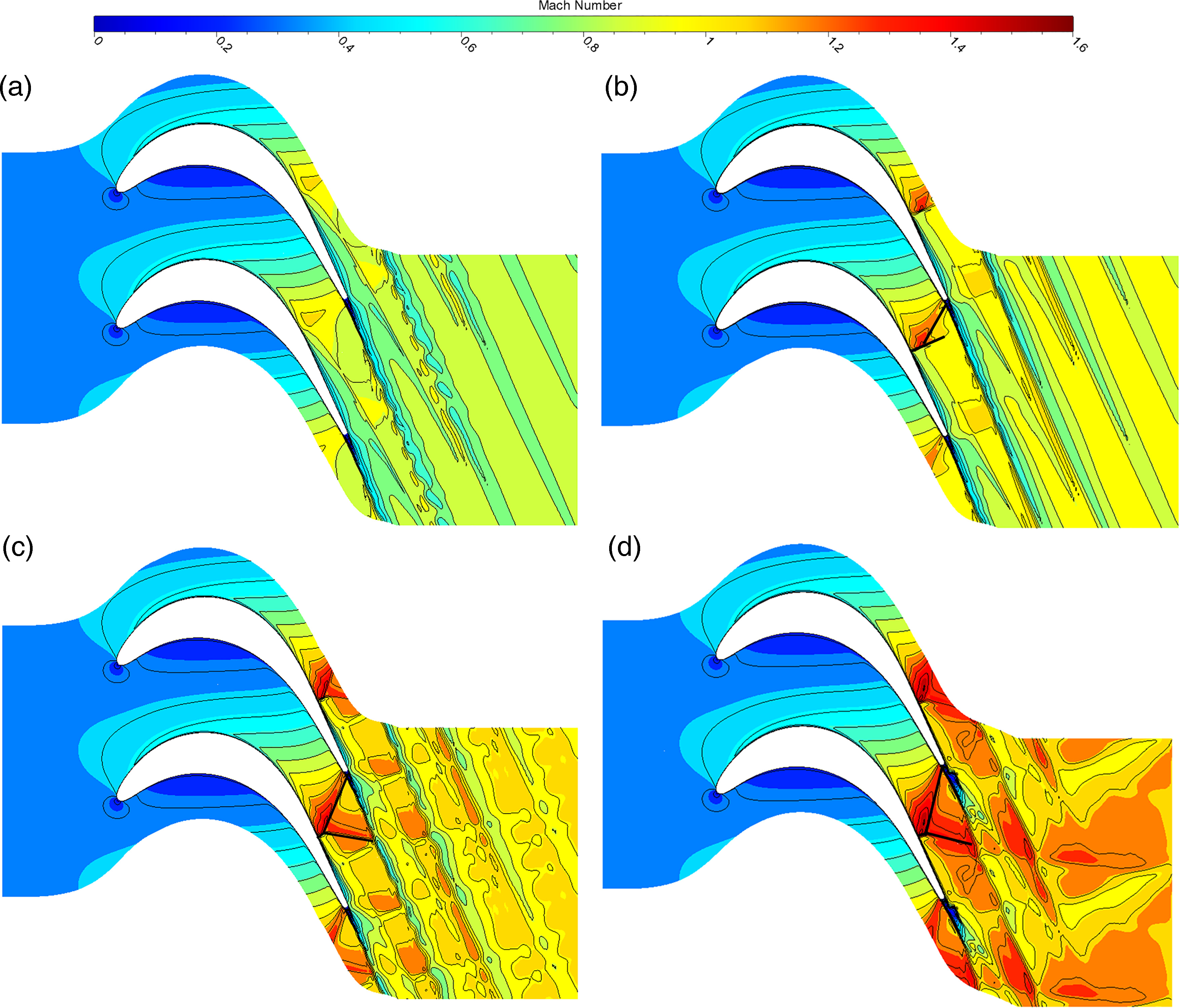
Figure 6.

Mach number contour at mid-span with different exit isentropic Mach numbers. (a) Exit isentropic Mach number 0.9 (b) Exit isentropic Mach number 1.0 (c) Exit isentropic Mach number 1.1 (d) Exit isentropic Mach number 1.2.

Figure 7.

Distribution of Cp at mid-span with different exit isentropic Mach numbers.

where P is the local static pressure, P1 is the exit static pressure and P0∗ is the inlet total pressure.

As Figure 6 shown, there is no shock wave formation at exit isentropic Mach number of 0.9. With the increase of the exit isentropic Mach number, the shock waves are generated, consisted of incident shock wave, reflected shock wave and Mach stem and the Mach number preceding the shock wave increases. The position of the shock wave at the suction surface moves towards the trailing edge and the angle between incident shock wave and reflected shock wave increases.

With the increase of exit isentropic Mach number, the sudden Cp rise in suction surface decreases in Figure 7, but the sudden static pressure rise increases according to the definition of Cp because of the difference of the inlet total pressure, which is induced by the shock wave and boundary layer interaction, indicating the intensity of the shock wave increases.

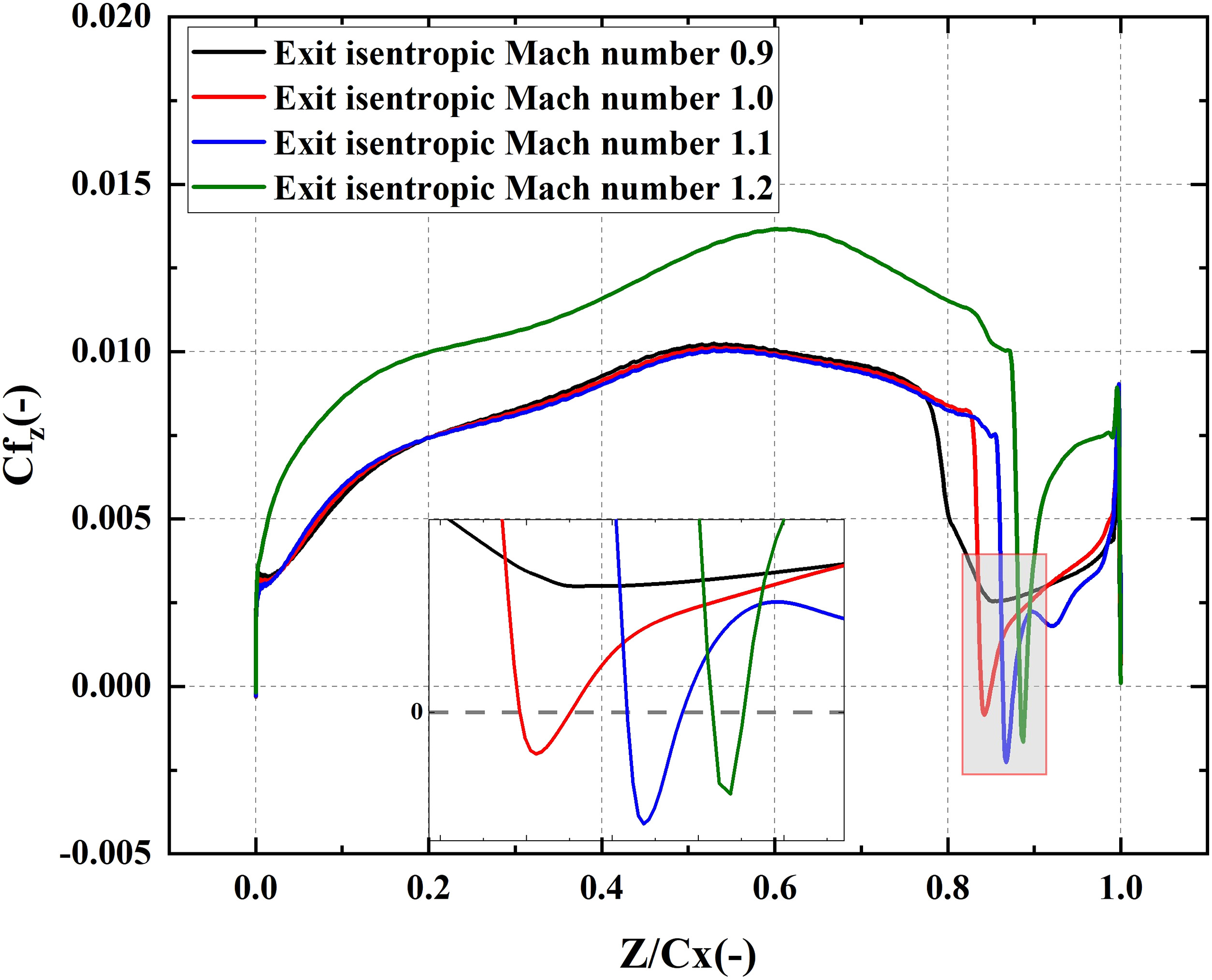
Figure 8 shows the distribution of axial skin friction coefficient (Cf_z) on the suction surface at mid-span. The axial skin friction coefficient is expressed by Equation 4.

Figure 8.

Distribution of Cf_z at mid-span on suction surface with different isentropic Mach numbers.

where τωz is the local axial wall shear stress, ρref and Vref are the reference density and reference velocity, respectively, for which the average inlet density and the average inlet velocity are used.

Cf_z can be used to represent the state of the boundary layer. The Cf_z less than 0 indicates there is a backflow region on the suction surface of the blade. The point of separation and reattachment of the flow is represented by the Cf_z of 0, which can be used to calculate the length of the separating bubble. In Figure 8, the Cf_z increases on the suction surface indicating that the boundary layer transitions from laminar to turbulent flow. The Cf_z suddenly drops to less than zero at the location where the shock wave occurs, which represents the point of separation. At various exit isentropic Mach numbers, the location of the separation bubble matches that of the shock wave, which moves towards the trailing edge. There is no separation bubble formation at exit isentropic Mach number of 0.9 and the length of the separation bubble increases from 1.18% to 1.29% Cx as the exit isentropic Mach number increases from 1.0 to 1.1. However, the length of the separation bubble is 0.73% Cx at the exit isentropic Mach number of 1.2, which is less than that at lower exit isentropic Mach number. It appears to show that the length of separation bubble does not grow as the intensity of the shock wave increases. The characteristics of the separation bubble at mid-span will be influenced by the secondary flow from the endwall as the exit Mach number increases.

Comparison of flow fields with different loading coefficients

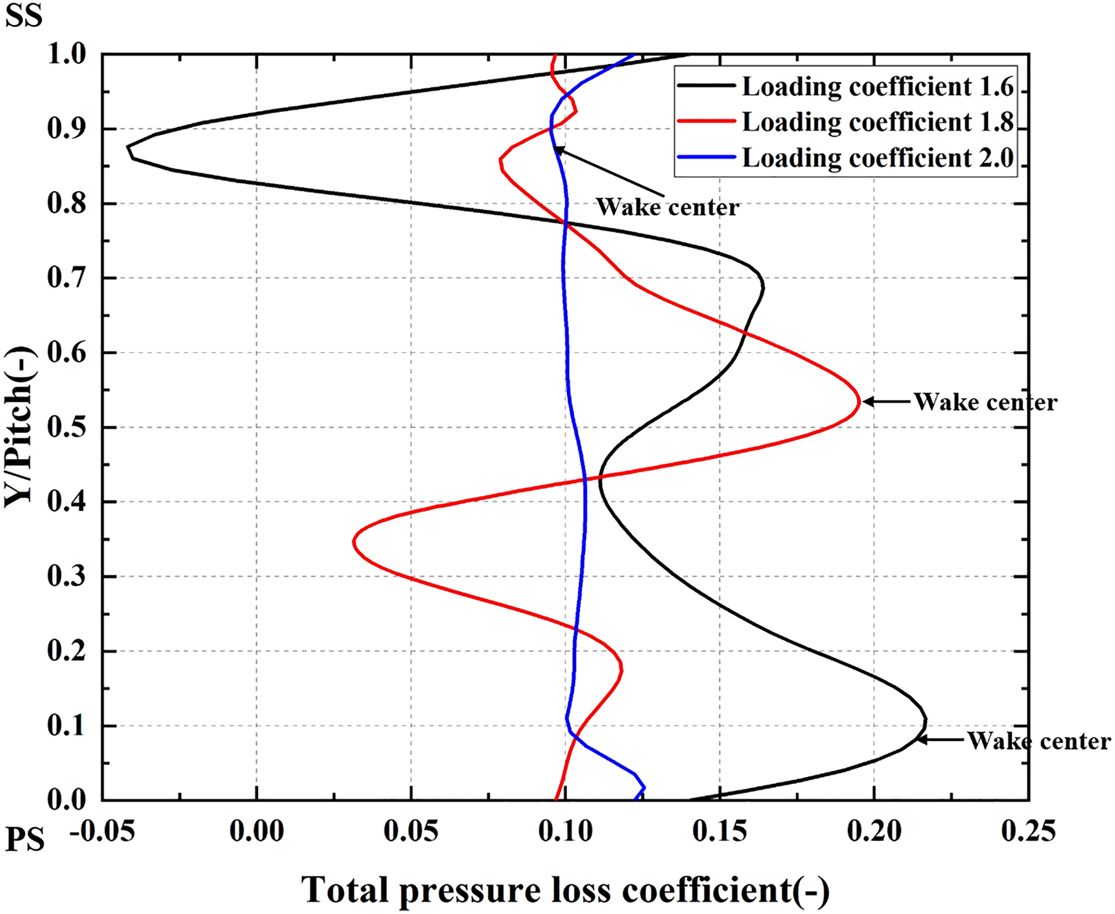
Figure 9 shows the total pressure loss coefficient at exit at exit isentropic Mach number of 1.2 and incidence angle of 0° with different loading coefficients. The total pressure loss coefficient reaches the maximum value of 0.097 at loading coefficient of 2.0 and reaches the minimum value of 0.090 at loading coefficient of 1.8 indicating there is not significant difference in the total pressure loss coefficient. Figure 10 shows the total pressure loss coefficient along pitch at exit of mid-span with different loading coefficients. The distribution of the total pressure loss coefficient and the position of the wake are different when the loading coefficient increases from 1.6 to 2.0 because the change in the loading coefficient is achieved by changing the turning angle. There is a high loss region corresponding to the wake at load coefficient of 1.6 and 1.8 and there is another high loss region at 0.7 pitch caused by the SWBLI at load coefficient of 1.6.

Figure 9.

Total pressure loss coefficient at exit with different loading coefficients.

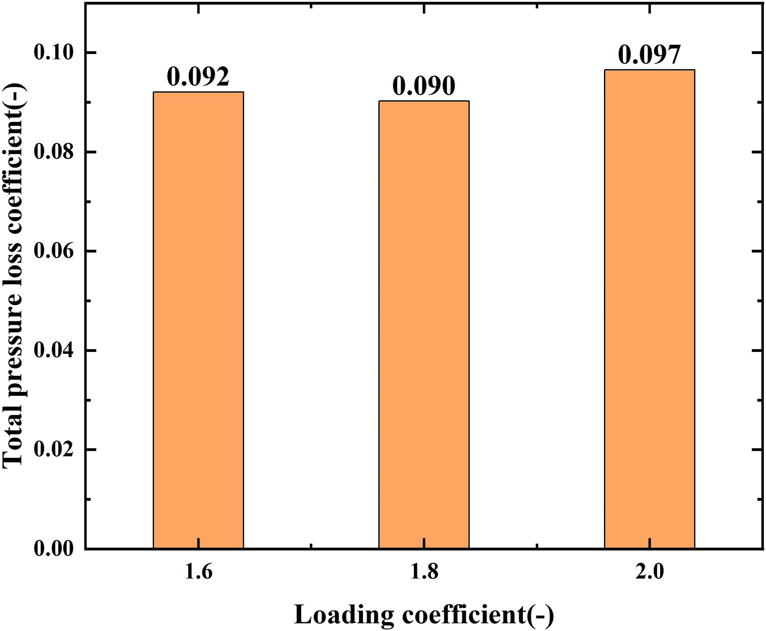
Figure 10.

Total pressure loss coefficient along pitch at exit of mid-span with different loading coefficients.

Figures 11 and 12 show the distribution of Mach number and Cp at mid-span. With the increase of the loading coefficient, the position of the shock wave moves towards the leading edge and the interaction between the shock wave and the wake strengthens, resulting in the uniformity of outlet flow field as the Figure 11 shown. The Mach number preceding the shock wave at load coefficient of 1.6 is significantly higher than others. Figure 12 shows the same change of the position of the shock wave and the Cp rise induced by the shock wave. The sudden Cp rise induced by the shock wave at load coefficient of 1.6 is higher than others, indicating the intensity of the shock wave is higher than others.

Figure 11.

Mach number contour at mid-span with different loading coefficients. (a) loading coefficient 1.6 (b) loading coefficient 1.8 (c) loading coefficient 2.0.

Figure 12.

Distribution of Cp at mid-span with different loading coefficients.

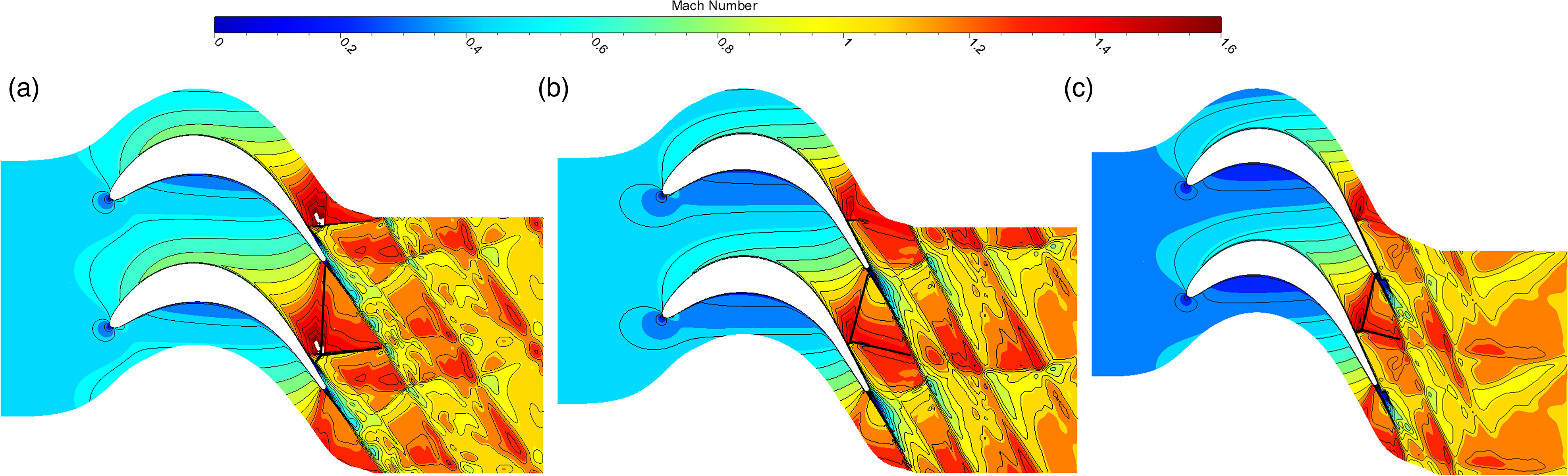
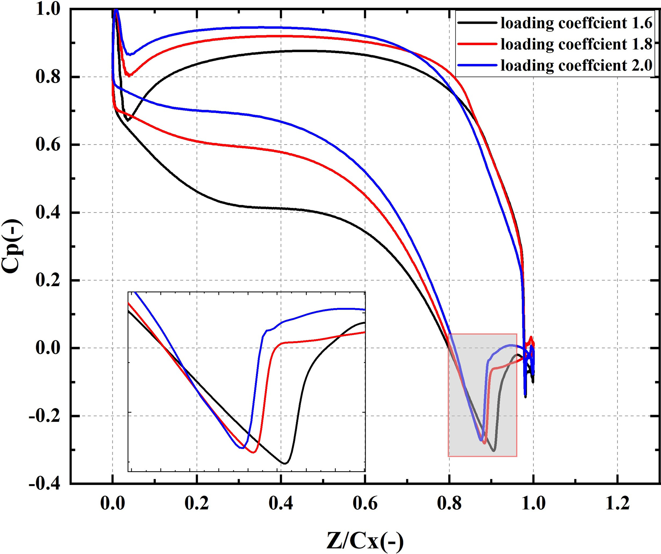
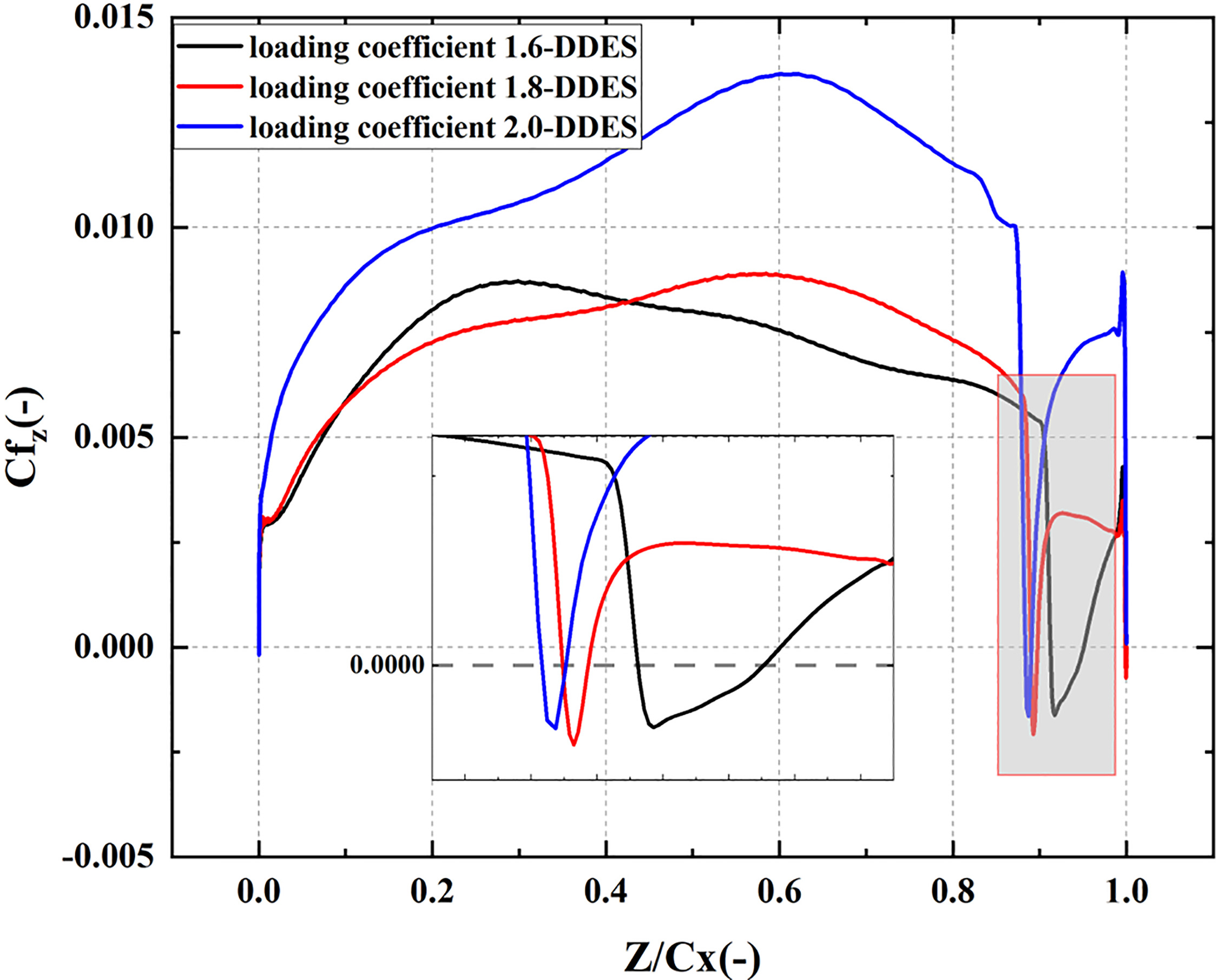
Figure 13 shows the distribution of Cf_z on the suction surface at mid-span. The transition at loading coefficient of 1.6 is completed earlier than that at the loading coefficient of 1.8 and 2.0. The length of the separation bubble induced by the shock wave is obviously longer than others at loading coefficient of 1.6, which leads to the higher total pressure loss coefficient at loading coefficient of 1.6 than at load coefficient of 1.8. With the increase of the loading coefficient, the length of the separation bubble decreases from 3.8% to 0.73% Cx.

Figure 13.

Distribution of Cf_z on suction surface at mid-span with different loading coefficients.

Comparison of flow fields with different ancidence angles

Figure 14 shows the total pressure loss coefficient at exit at loading coefficient of 2.0 and exit isentropic Mach number of 1.2 with different incidence angles. The total pressure loss coefficient reaches the maximum value of 0.119 at incidence angle of +15° and reaches the minimum value of 0.091 at incidence angle of negative 7.5°, indicating the loss increase with the large positive incidence angle. Figure 15 shows the total pressure loss coefficient along pitch at exit of mid-span with different incidence angles. At the negative incidence angles, there is a high loss region at 0.94 pitch corresponding to the wake and there is another high loss region at 0.6 pitch because of the flow separation induced by the SWBLI. The distribution of the total pressure loss coefficient at incidence angle of 0° is basically uniform because of the strong blend of the main flow and the wake. There is a high loss region at 0.94 pitch corresponding to the wake at incidence angle of positive 7.5°, however, the distribution is absolutely different at incidence angle of positive 15°. The high loss area is generated by separated flow from the suction surface, not by the wake.

Figure 14.

Total pressure loss coefficient at exit with different incidence angles.

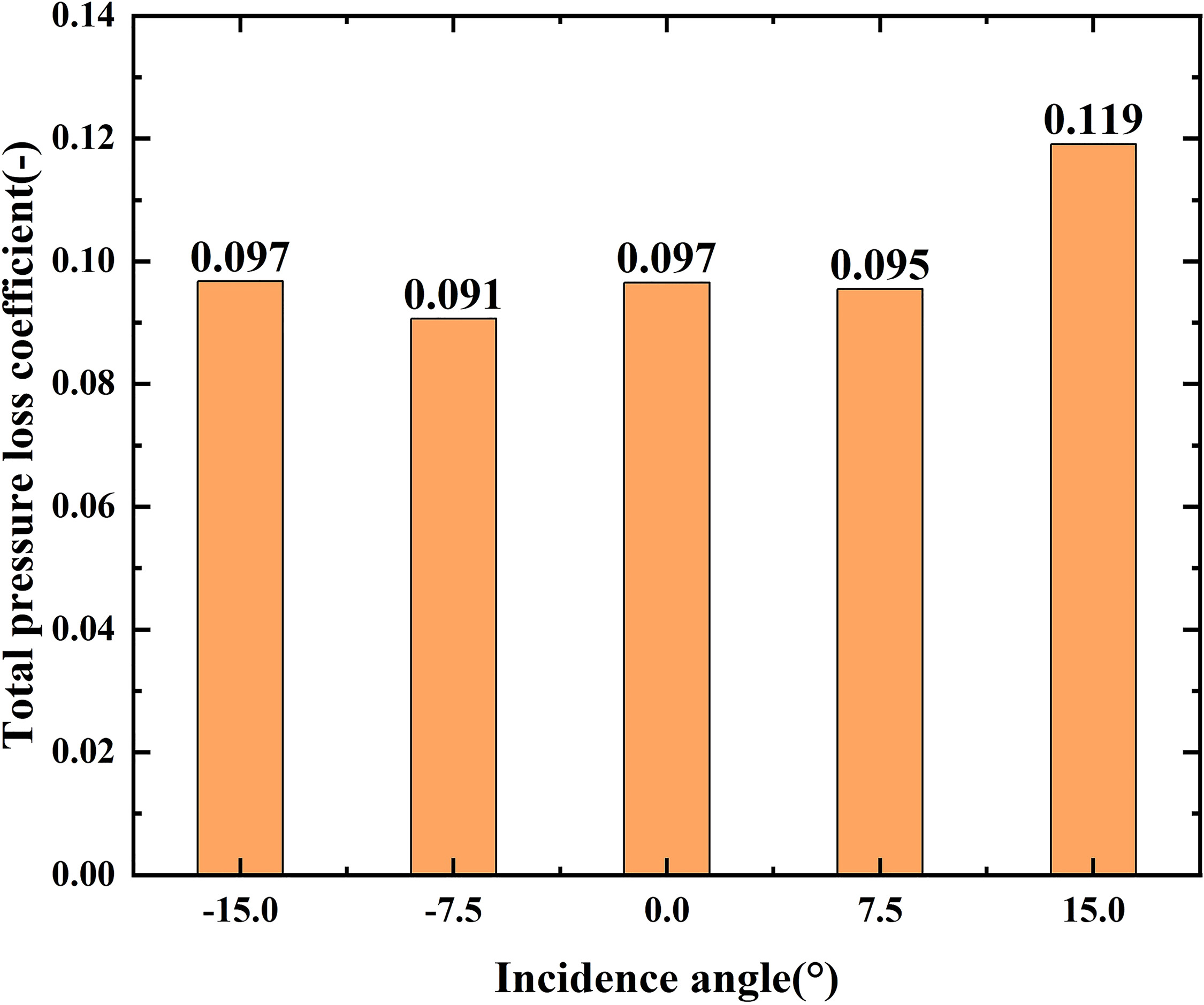
Figure 15.

Total pressure loss coefficient along pitch at exit of mid-span with different incidence angles.

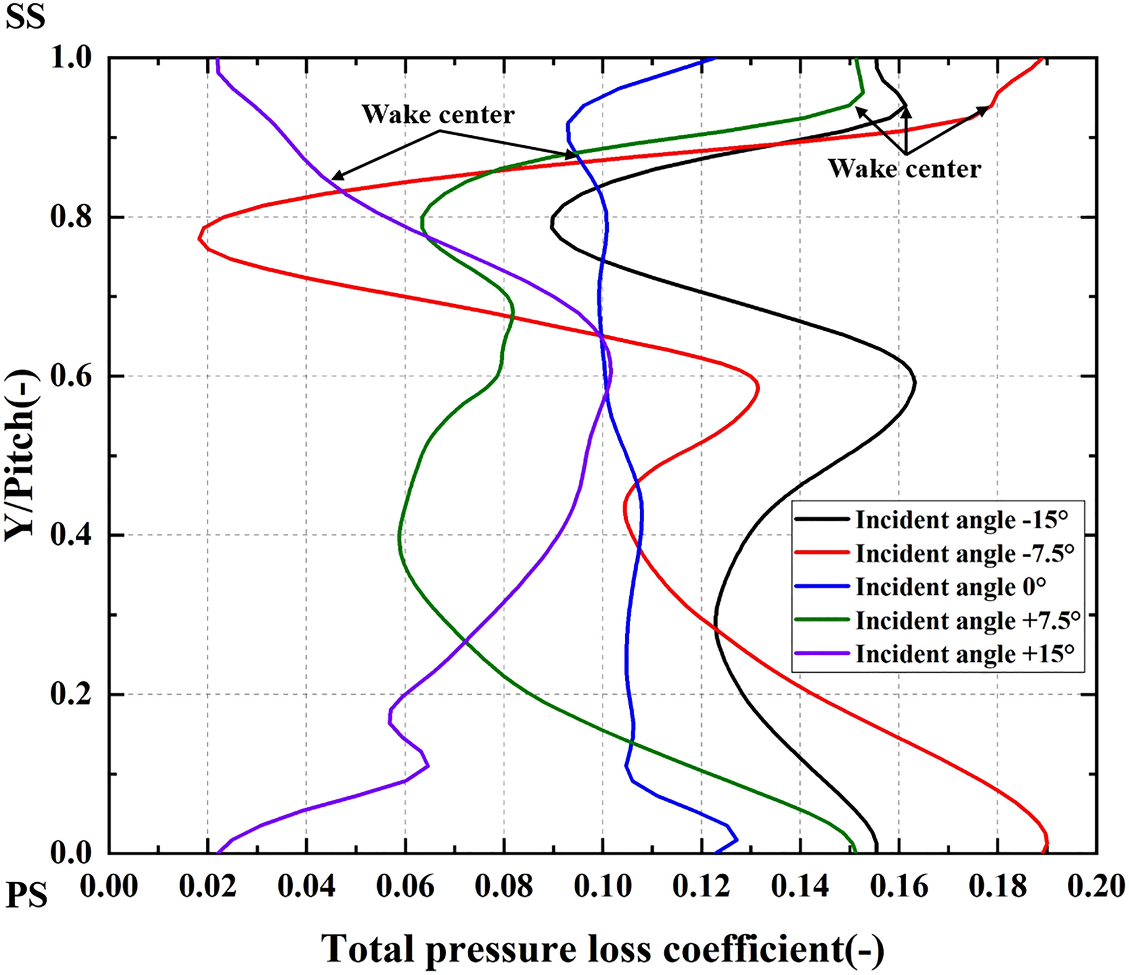
Figure 16 shows the distribution of Mach number at mid-span. There is a large flow separation on pressure surface at incidence angle of −15° and a large flow separation on suction surface at incidence angle of +15°. The large flow separation on pressure surface at incidence angle of −15° does not influence the trailing edge shock wave. The structure of the shock wave and the flow field are similar with different incidence angles except the incidence angle of +15°. There is the shock wave at the leading edge of the suction surface at incidence angle of +15° resulting in the large flow separation, the bending of the shock wave at the trailing edge and the increase of the loss. The intensity of the wake and the interaction between the shock wave and the wake are reduced, leading to the different distribution of the total pressure loss coefficient as Figure 15 shown.

Figure 16.

Mach number contour at mid-span with different incidence angles. (a) Incidence angle −15° (b) Incidence angle −7.5° (c) Incidence angle 0° (d) Incidence angle +7.5° (e) Incidence angle +15°.

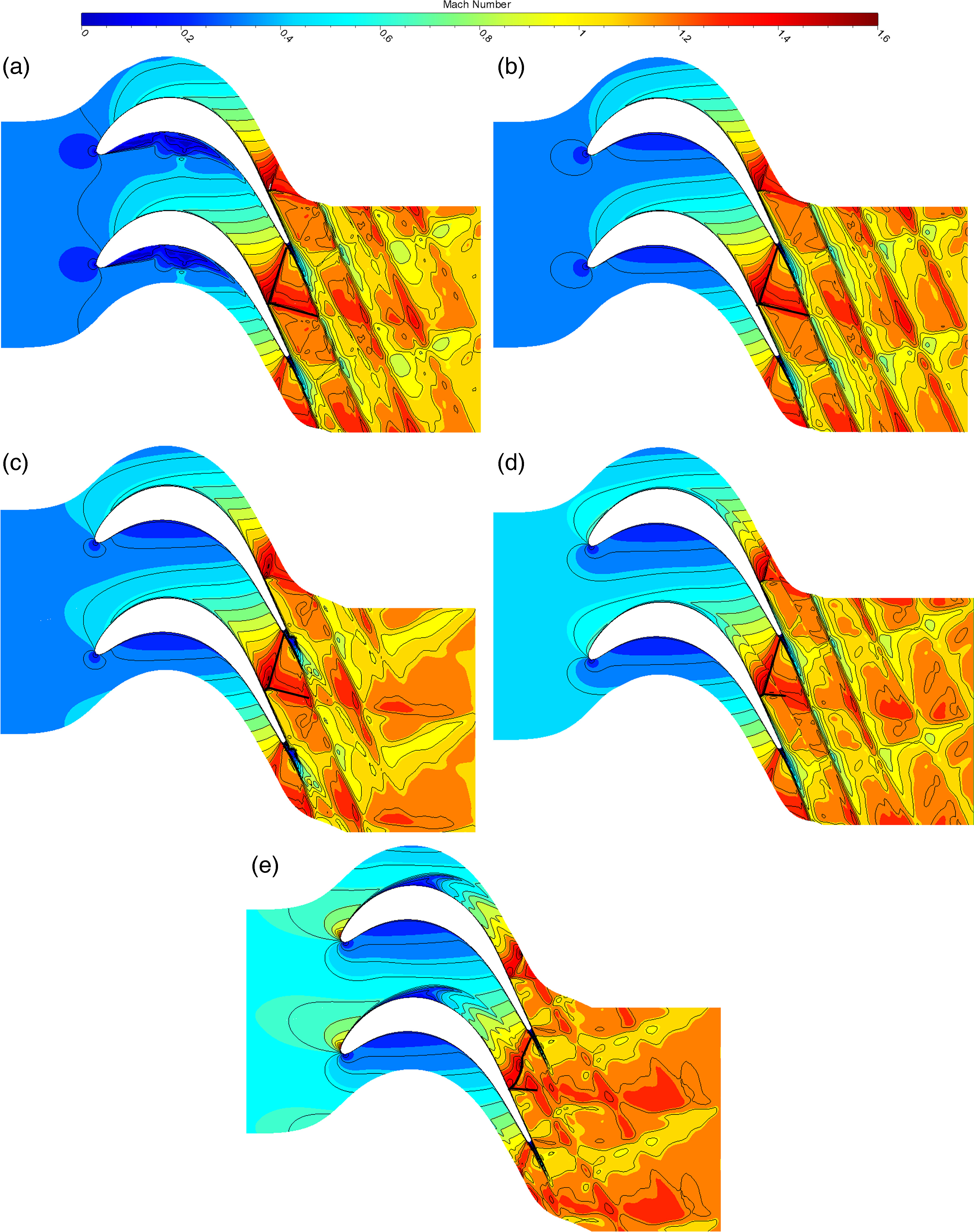
Figure 17 shows the distribution of Cp at mid-span. With the variation of the incidence angles, the position and the intensity of the sudden Cp rise induced by the shock wave are essentially the same but the intensity of the sudden Cp rise at the incidence angle of +15° significantly increases because the shock wave is bent and is more perpendicular to the direction of the flow. Additionally, there is a sudden Cp rise at the leading edge of the suction surface representing the formation of the shock wave.

Figure 17.

Distribution of Cp at mid-span with different incidence angles.

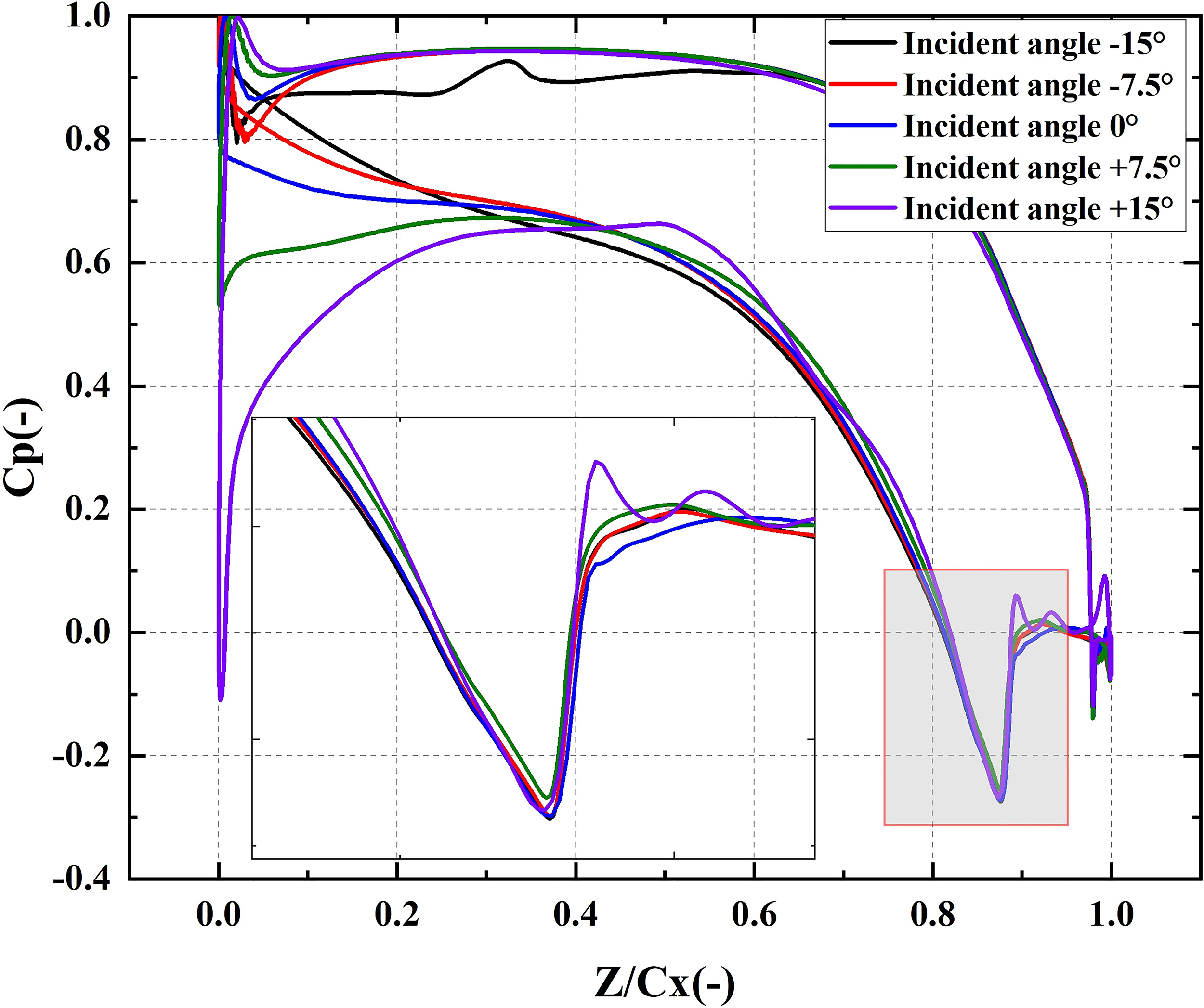
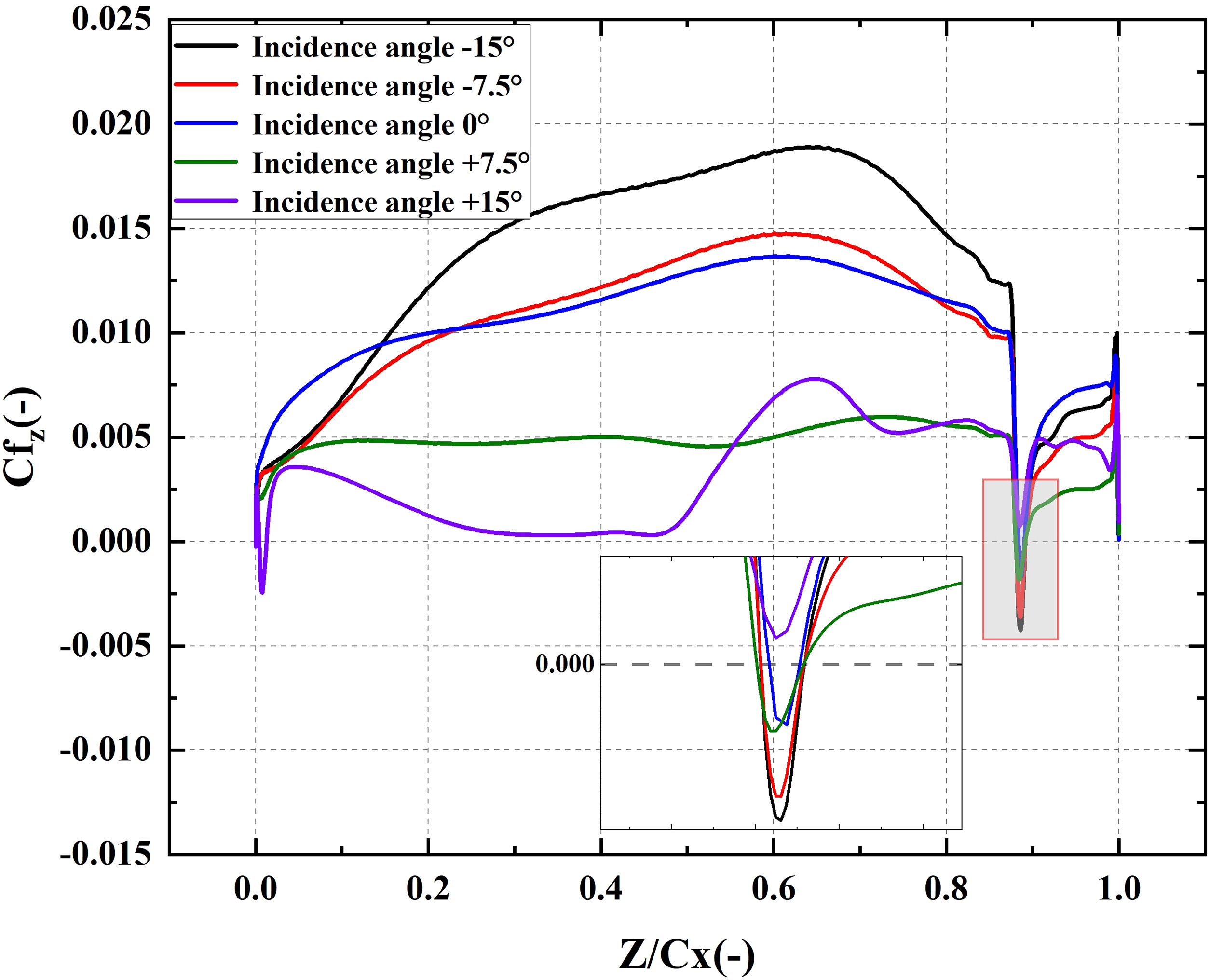
Figure 18 shows the distribution of Cf_z on the suction surface at mid-span. The Cf_z quickly drops when the shock wave occurs on the suction surface and the separation bubble is generated with diffident incidence angles except the incidence angle of +15°. At the incidence angle of +15°, the boundary layer at the trailing edge of the suction surface thickens but no separation bubble is generated because there is a separation bubble formation with the length of 0.8 Cx at the leading edge of the suction surface. As the flow develops, the open separation occurs following the separation bubble as the Figure 16 shown. The position of the separation bubble is almost the same and corresponds to the position of the shock wave at other incidence angles. The length of the separation bubble is 1.11% Cx at negative incidence angles, 0.73% Cx at the incidence angle of 0° and 1.12% Cx at the incidence angle of +7.5°.

Figure 18.

Distribution of Cf_z on suction surface at mid-span with different incidence angles.