Introduction
The study of the dynamic behavior of turbine bladed disks vibration is still a topic of great importance. When the excitation frequency is close to a natural frequency of the system, within the engine speed working range, the vibration amplitude can lead to high-cycle fatigue failure. Friction damping devices such as UPDs are typically included into turbine design to limit these resonant vibrations (03, 05). Each damper is pressed against the blade platforms by the centrifugal force. When relative motion takes place between damper and blade platform, the generated nonlinear friction forces lead to the dissipation of vibrational energy. From an industrial point of view, it is fundamental to have effective tools for the design and performance prediction of UPDs. In the last 20 years different authors worked on this topic and proposed several numerical models, they can be found, among the others, in the papers by (22, 26, 11, 14).
The basic idea is that the calculation of the nonlinear forced response is performed by coupling the UPD to the blades modelled through FE. This coupling is achieved by inserting a contact element between blades and UPD. The contact element is characterized by four parameters, which must be chosen by the user: the friction coefficient, the normal contact stiffness and the tangential contact stiffness in two perpendicular directions.
The problem of solving the nonlinear equation of the forced response in presence of contact forces, depending on the structure displacement, is nowadays completely overcome. The nonlinear forced response can be calculated with high computational efficiency in the frequency domain using the harmonic balance method (HBM) (23, 09, 10, 24, 14, 27, 25).
Being the calculation method well-established, the still open question is how to choose the contact parameters (friction coefficient, normal and tangential contact stiffness) in order to obtain reliable predictions of the forced response. In literature contact parameters are usually tuned by matching the computed forced response function (FRF) with the measured one. This method, however is not a viable procedure at the design stage, where experimental FRFs are not yet available.
This paper presents the numerical results obtained by a numerical code where the damper model, the contact model and the method for solving the equations are aligned with the state of the art. The attention is here focused on the procedure adopted for choosing contact parameters: only those procedures which do not rely on curve fitting between experimental and numerical FRFs are considered. The present paper adopts two such alternative ways to estimate contact parameters: the first is an established analytical model from the literature and the second is based on direct experimental measurements (i.e. hysteresis cycles) on UPDs on a dedicated test rig. The chosen test case is a bladed disk carrying cylindrical UPDs. The comparison between measured FRFs and simulated ones will highlight strengths and limitations of each method used for contact parameter estimation.
Bladed disk with underplatform dampers
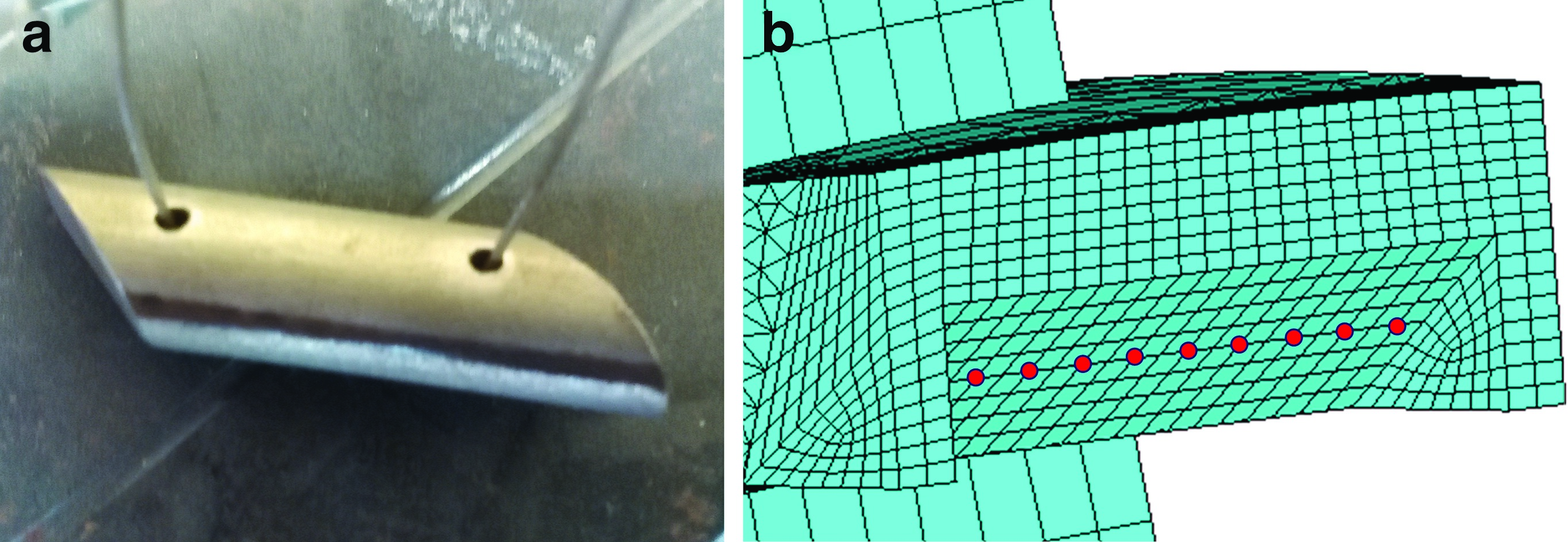
The test case analyzed in this paper is the bladed disk (blisk) shown in Figure 1. The bladed disk carries between each couple of blades a cylindrical UPD, sketched in Figure 2 and shown in Figure 10. This blisk and the UPDs were chosen as a test case since they are part of a test rig (Octopus test rig) (04, 13) that provides experimental forced response of blisks with UPDs under controlled conditions.

Nonlinear dynamic equilibrium equation
The reduced mass and stiffness matrices of the bladed disk are exported from the FE code in Matlab and they are used for the calculation of the dynamic forced response of the blisk using a dedicated in-house numerical code.
Dynamic equation of the bladed disk
The dynamic equations of the bladed disk in the time domain are nonlinear second order differential equations:
where M, K are the reduced mass and stiffness matrices (12), C is the damping matrix, linear combination of M and K,
where Nh is the retained number of harmonics, n = 0…Nh and ω is the frequency of the excitation forces. By substituting –– into the general balance , the initial nonlinear second order differential equations are turned in the frequency domain into a set of nonlinear algebraic complex equations:
where
Dynamic equations of the damper
The damper is considered as a rigid body with inertia properties. The damper equilibrium equation in the time domain is:
where
where Nh is the retained number of harmonics,
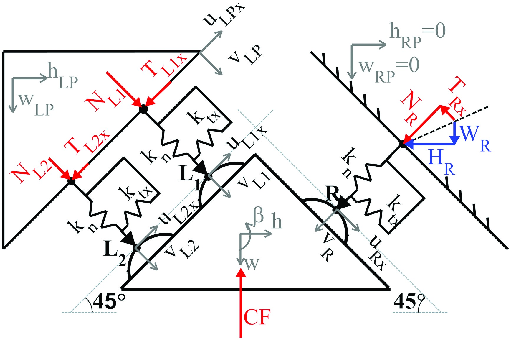
Contact model
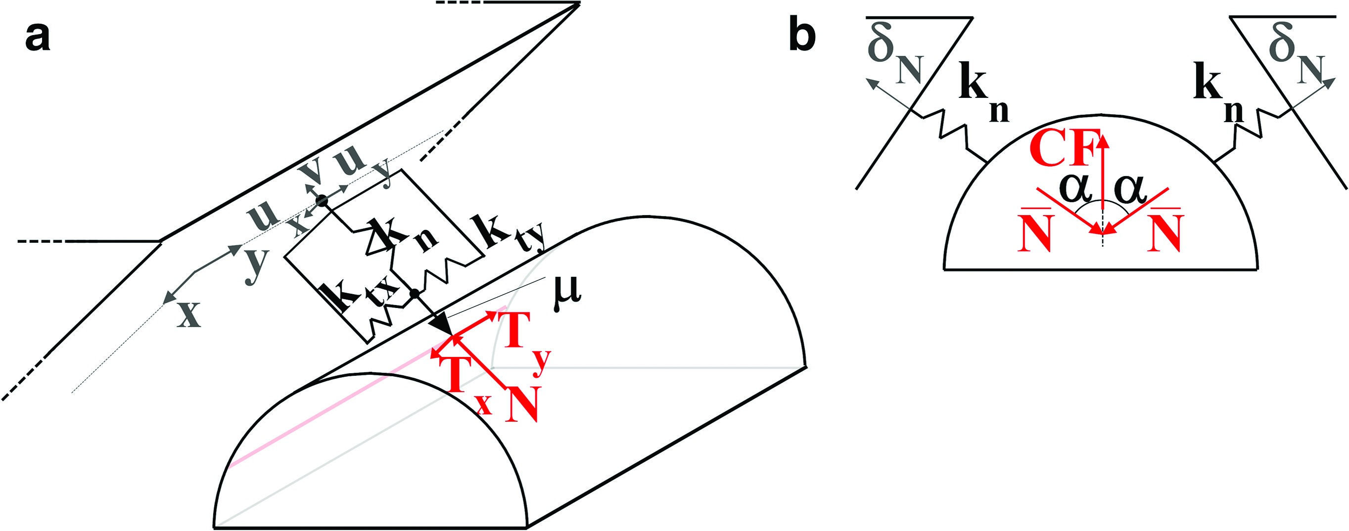
The contact model, a typical macroslip element, takes into account a two-dimensional tangential relative displacement and a variable normal load. The contact model applied to a contact point on the damper is sketched in Figure 2.
The plane (x,y) is tangent to the UPD and represents the surface of the blade platform. Two springs define the tangential contact stiffnesses
Determination of contact parameters
A key point for a correct calculation of the forced response in presence of UPDs is the choice of the correct contact parameters (contact stiffness and friction coefficient) to be given as input to the contact model.
There are analytical methods in literature (07, 18, 01, 02) to calculate the contact stiffness values in normal and tangential direction starting from the geometry and the material of the UPD. The same contact stiffness values can also be determined from measurement of forces and displacement but only on dedicated test rigs.
Some focus on single flat-on-flat contacts under constant normal loads and high temperatures (21, 06, 20), and are therefore not useful in this specific case. On the other hand, the Damper Test Rig (17) aims at estimating contact parameters of UPDs (cylinder-on-flat interfaces as well) under more realistic working conditions in terms of variable normal load and complex interface kinematics.
The friction coefficient cannot be calculated with the analytical technique presented here, it is therefore measured. These different approaches for the choice of the contact parameter values are here presented.
Analytical calculation of the contact stiffness values
Normal contact stiffness
The normal load N at the contact line causes an elastic deformation
where
01and02 use the pressure distribution to compute the normal relative displacements of the contact surfaces by means of the Cerruti potential theory (19):
where
The value of the normal contact stiffness is obtained by taking the derivative of the normal penetration
Hence,
In the last equation, the dependence on the normal load N is hidden in b, half-width of the contact area, function of N.
–, are here applied to the cylindrical UPD of Figure 2 where the length is L = 27.6 mm and the radius of the cylinder is R = 5 mm. The length of contact corresponds to the nominal length of the UPD, as shown by the wear marks (see Results section). The half-width of the contact area
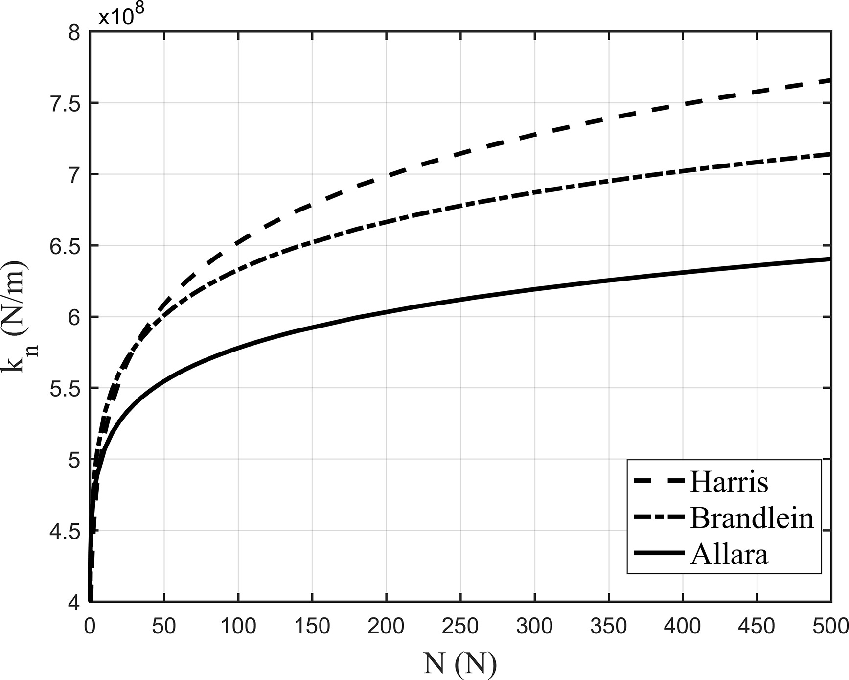
Figure 3 shows that the three analytical models lead to three different plots. It will be observed later however that this discrepancy does not significantly influence the calculated FRFs of blades with damper: it leads to a difference lower than 1.5% in the frequency value of the blades with damper when the different
Tangential contact stiffness
The cylindrical UPD, in contact with the blade platforms, undergoes contact forces and displacements in the tangential direction.
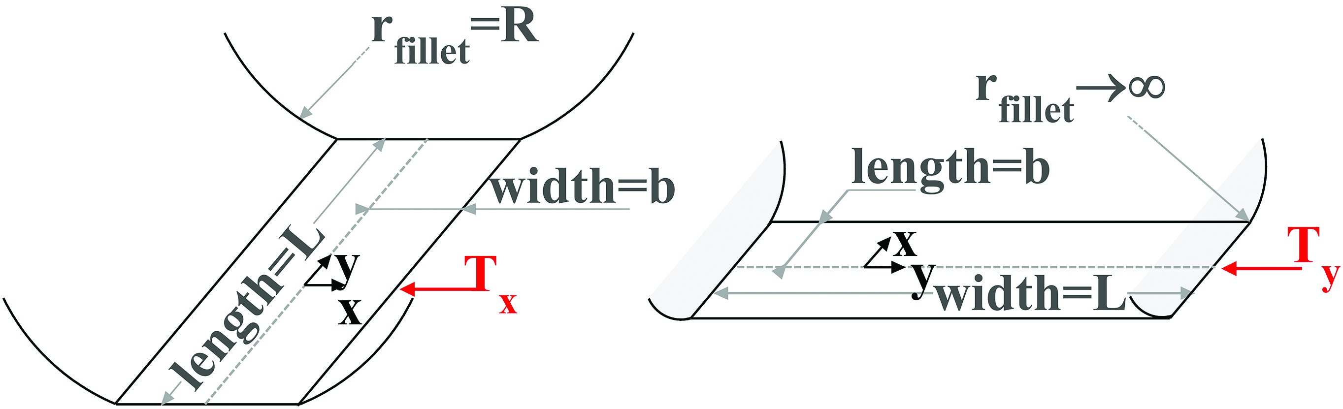
01and02 found the analytical expression for the monotonic loading curves and hysteresis cycles (i.e. contact forces vs. relative displacement) of a filleted flat punch pressed against an infinite half-plane. The flat punch can be customized with material properties and contact area width, length and fillet radius. As shown in Figure 4 this parameter setting can be used to reproduce the case of a cylinder pressed against a plane moving alternatively along the x direction (Figure 4) and the y direction (Figure 4) to determine respectively
Experimental estimation of the contact stiffness values
Contact stiffness values
The test rig shown in Figure 6, developed over the years by the AERMEC laboratory (see 17 for a detailed description), is designed aiming at:
Figure 6.
(a) Damper test rig photo and measured quantities, displacements in white, forces in blue. (b) Example of hysteresis cycle time evolution.
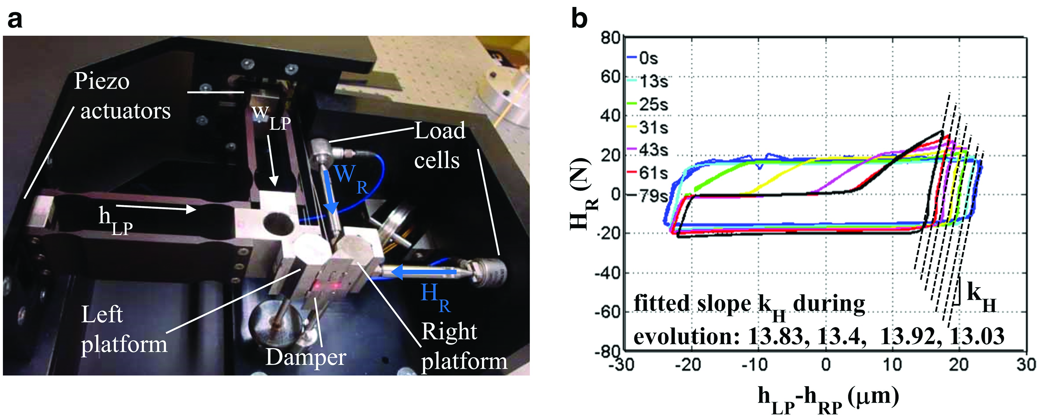
1. imposing user-defined in-plane displacements simulating the so-called In-Phase (IP, vertical) and Out-of-Phase (OOP, horizontal) relative motion between the blades platforms by means of two piezo-actuators connected to the left dummy platform;
2. measuring the forces transmitted between the two platforms through the damper by means of two load cells connected to the right dummy platform.
Please notice that all measured quantities are reported both in Figure 5 and in Figure 6. Relative platforms displacements, measured using a laser head, are plotted against the corresponding component of the contact force (“hLP vs. HR” in case of OOP motion and “wLP vs. WR” in case of IP motion) in the global damper hysteresis cycle. The evolution of a typical OOP hysteresis cycle is shown in Figure 6. The slope kH highlighted in Figure 6 keeps constant throughout the evolution approximately equal to and corresponds to specific contact state: all contact points (R, L1 and L2) are repeatedly in stick condition, as confirmed by additional experimental evidence and numerical results in 0 (17). The fitted slope kH is therefore a composite effect of normal and tangential stiffness values at all contacts
Table 2.
Total contact stiffness.
| Method | kn | ktx | kty |
|---|---|---|---|
| Analytical | 5.50·108 | 5.71·108 | 6.07·108 |
| From measurements | 5.53·108 | 1.70·107 | 1.70·107 |
The procedure described above does not provide an estimate of the tangential contact stiffness
Table 1.
Frequency values in stuck condition using contact stiffness values estimated experimentally.
| Stuck peak frequency (Hz) | Stuck peak amplitude (m/s/N) | |
|---|---|---|
| 143.8 | 0.548 | |
| 144.9 | 0.531 | |
| 150.3 | 0.528 |
It can be observed that the sensitivity of frequency and amplitude of the stuck peak to variations of

Determination of the friction coefficient
The value of the friction coefficient was measured through ad hoc experimental measurements as described in (15). A value of 0.6 was measured at room temperature over a range of 5·106 cycles. Furthermore, the measurements in (Lavella et al., 2013) match with the stabilized values of friction coefficients for cylindrical contacts measured on the dedicated damper rig (15).
Experimental Results
Experimental results of the forced response measurements are available from the Octopus test rig described by 04 and 13. A selection of experimental FRFs are here compared with the calculation results in order to check whether each choice of contact parameters is correct.
Description of the test rig
Figure 7 shows the Octopus test rig. The bladed disk (1), is fixed to a support (2). The arm structures (3) hold one pulley each, they are mounted on the external ring (4) equally spaced around the circumferential disk direction. The simulation of the centrifugal force on each UPD is obtained by means of two wires (5), which pass over the arms and are connected through the pulley to a dead weight. The excitation system is a non-contact travelling wave generated by electromagnets below each blade as shown in Figure 7.
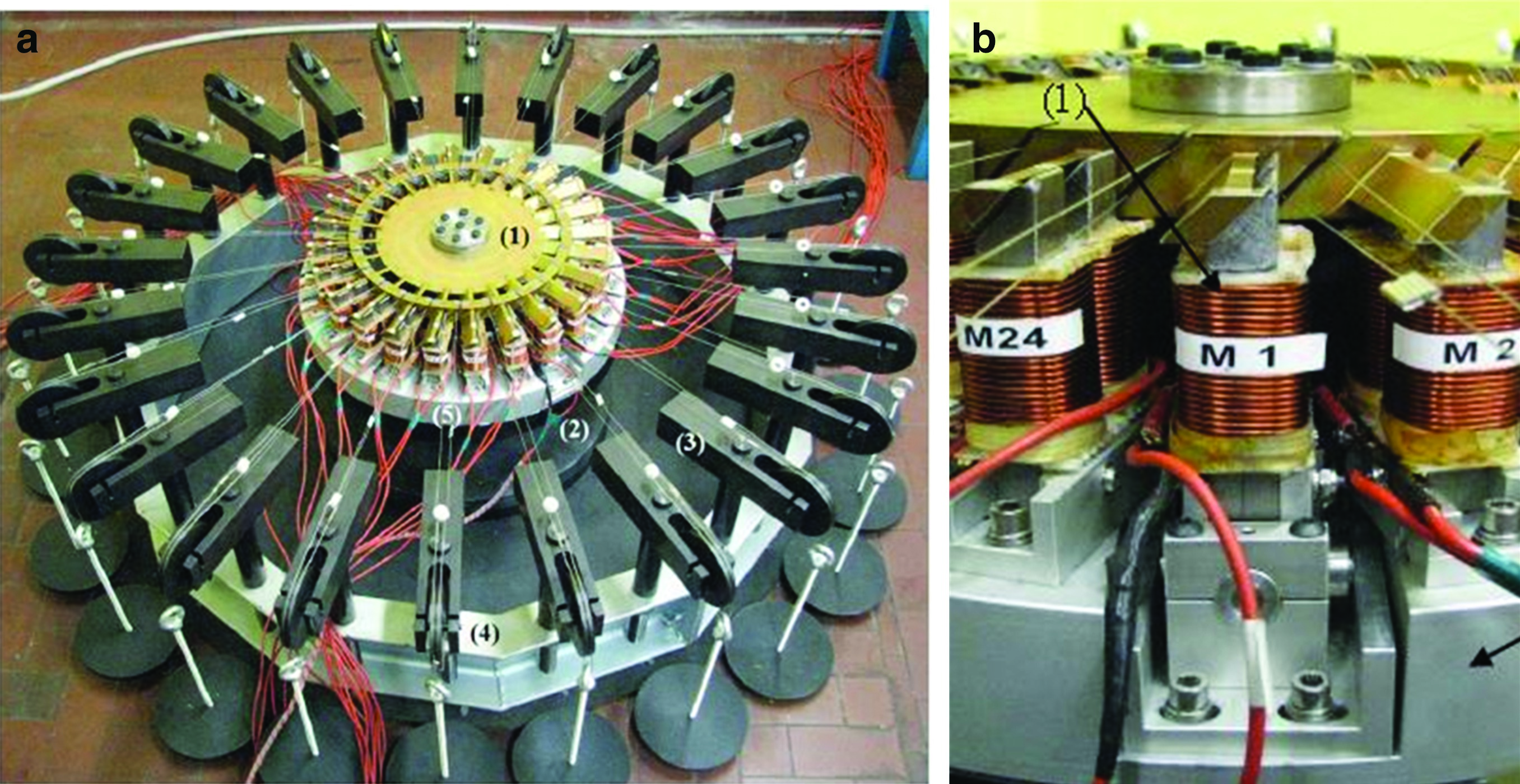
The electromagnets can be activated with a given phase shift in time in order to generate the required EO type excitation. The dynamic response of the disk is carried out by means of a laser scanning vibrometer. An example of measurement is shown in Figure 8 which shows the FRFs of the 24 blades excited by EO = 2, excitation force on each blade Fext = 0.3 N (where Fext =
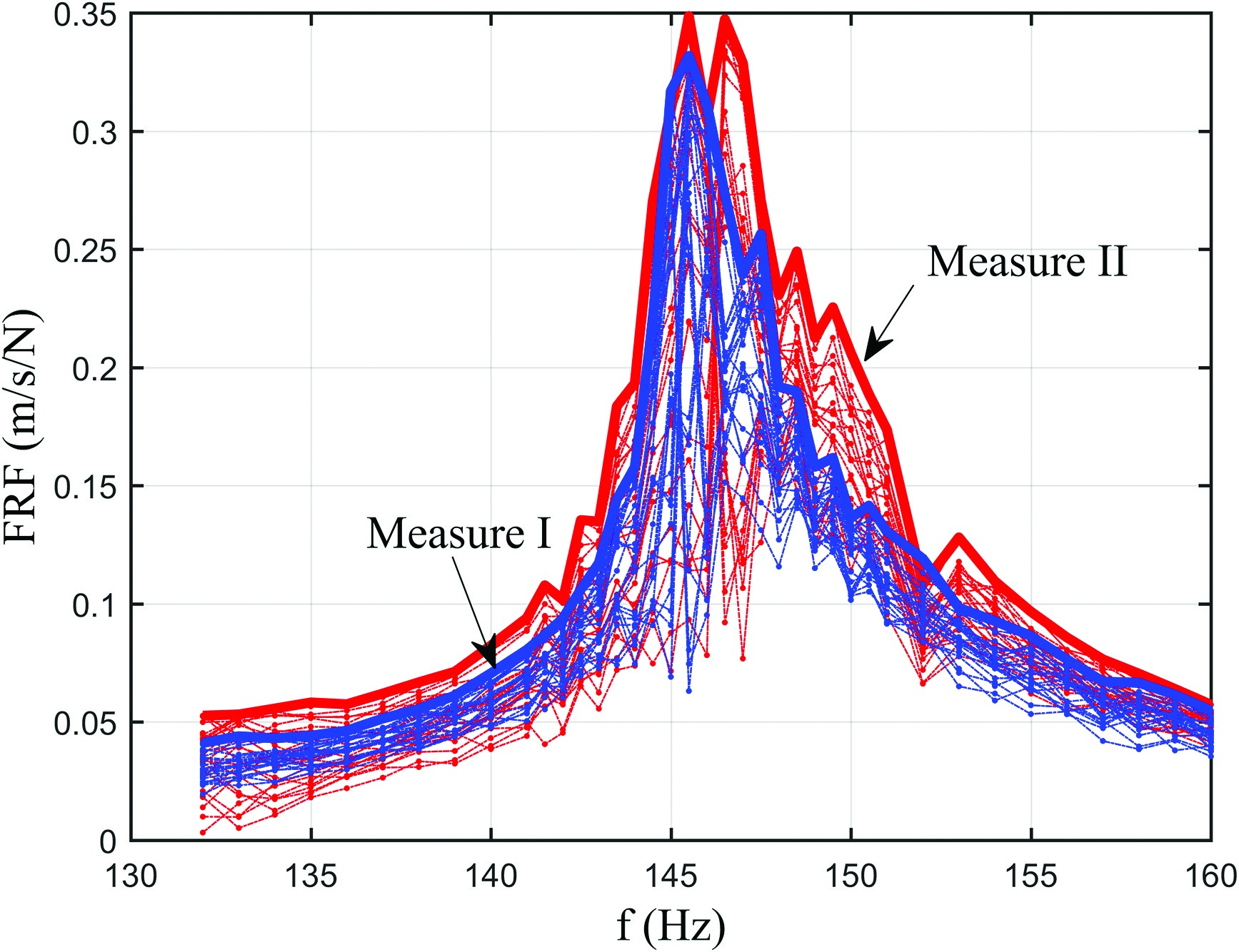
Post-processing of measured mistuned responses
It can be seen in Figure 8 that, due to the presence of small mistuning, defined as small variations between each disk sector as explained in (08), there is a difference between the FRFs of each blade. The bold red and blue lines are the envelope of the maxima of the FRFs at every frequency for the two sets of measurements. The envelope of the maxima represents the worst case working condition that is the maximum vibration amplitude for each frequency. The two curves representing the envelope of the maxima are not overlapped but they show that the maximum amplitude value and the resonance frequency value is in the same range for the two set of measurements. Similar FRFs are obtained for different excitation amplitude values. The two curves of the envelope of the maxima (an example is Figure 8) will be used as reference for comparison with numerical results.
Results and discussion
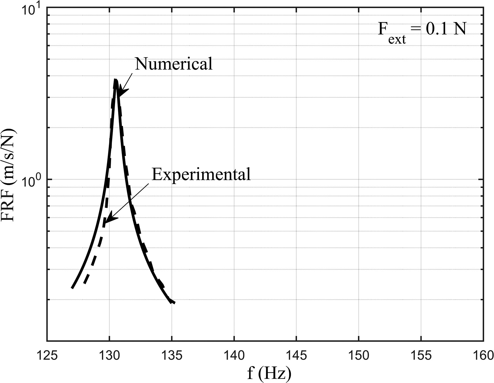
The numerical procedure described in the previous sections has been applied for the calculation of the forced response of the first bending mode (excitation type EO = 2) of the bladed disk. A numerical model becomes predictive thanks to a combination of factors. A representative FE model, the faithful representation of the boundary conditions and a numerical solver adequate to the application are considered as prerequisites. The soundness of the techniques mentioned above is demonstrated by the good matching between the numerical and experimental response of the disk without UPDs (i.e. linear case in Figure 9).
Other factors such as a trustworthy representation of contact conditions, achieved only through a deep knowledge of the contact parameters requires instead a novel approach, which is the focus of this paper.
The calculation with the UPDs requires the selection of contact nodes to which macroslip elements (contact forces) are applied. From the observation of the wear marks on the damper (as shown in Figure 10) it was deduced that the contact was along all the contact line cylinder-platform. The contact nodes were then selected along a line on the platform as shown in Figure 10. A contact model like that shown in Figure 2 was then applied to each contact node. The crucial point is the choice of the correct contact parameters since a wrong choice could lead to completely wrong results. As stated before the value of friction coefficient was assumed as 0.6 from previous measurements on a dedicated test rig (Lavella et al., 2013). The analytical set of contact stiffness assumed in the calculation is shown in the first row of Table 2. These contact stiffness values have still to be divided by the number of contact points. The value of kn in the first row of Table 2 is calculated by applying (07). The value of ktx and kty were calculated according to the Allara’s flat punch model of Figure 4. The calculation of the contact stiffness values requires the value of the contact normal load. During operation the normal load
On the same Table 2 in the second row, the contact stiffness values, coming from the data treatment of the measurements on the rig of Figure 6, are listed. The value of kty was assumed equal to ktx since it was not measured on the test rig. It can be observed that the calculated normal stiffness (kn) value matches with the measured value. On the contrary, the calculated tangential stiffness (ktx) is an order of magnitude lower the measured one. The FRF calculation results using as input the calculated stiffness values (first row of Table 2) are shown in Figure 11. The other input parameters are: centrifugal force on the damper is CF = 147 N, EO = 2, first bending mode, excitation force on each blade Fext = 0.2 N.
Figure 11.
Comparison between experimental and numerical FRFs. Fext = 0.2 N. Contact stiffness values estimated analytically.
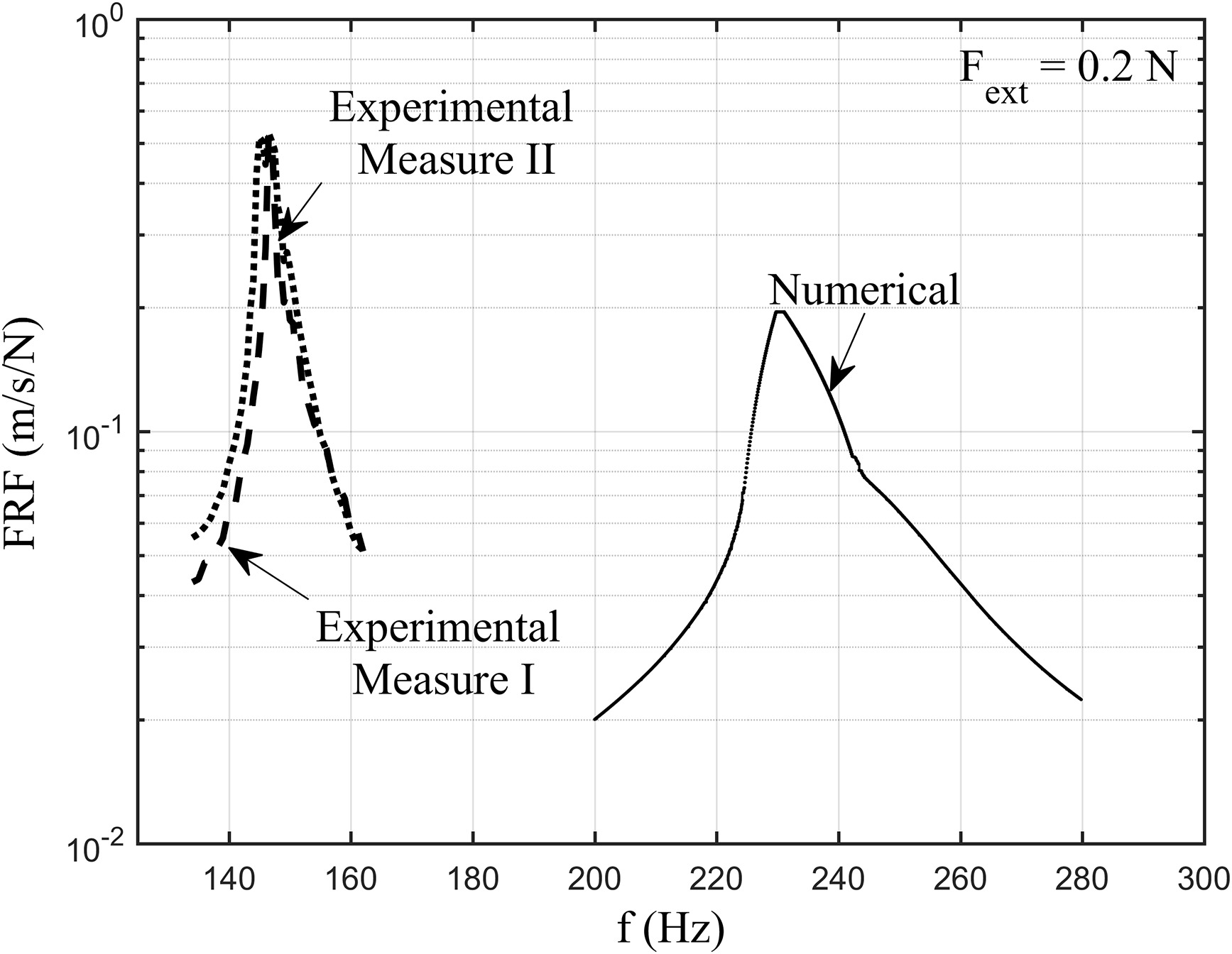
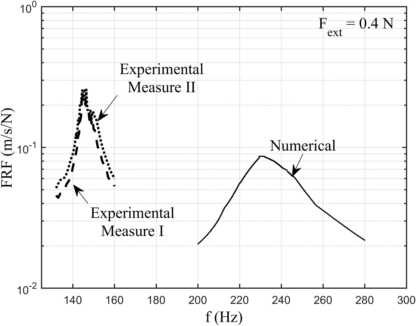
Figure 12 shows the results for the same case but with Fext =0.4 N. It can be observed how the calculated value of contact stiffness leads to FRFs where the resonance frequency is largely overestimated. The calculated FRF does not match with the experimental FRFs neither in terms of frequency nor in terms of amplitude. On the other hand, if the contact stiffness values coming from the measurement (second row of Table 2) are used as input in the calculation, the FRFs of Figure 13 and Figure 14 for the same two cases are obtained.
Figure 13.
Comparison between experimental and numerical FRFs. Fext = 0.2 N. Contact stiffness values estimated through direct experiments on dampers.
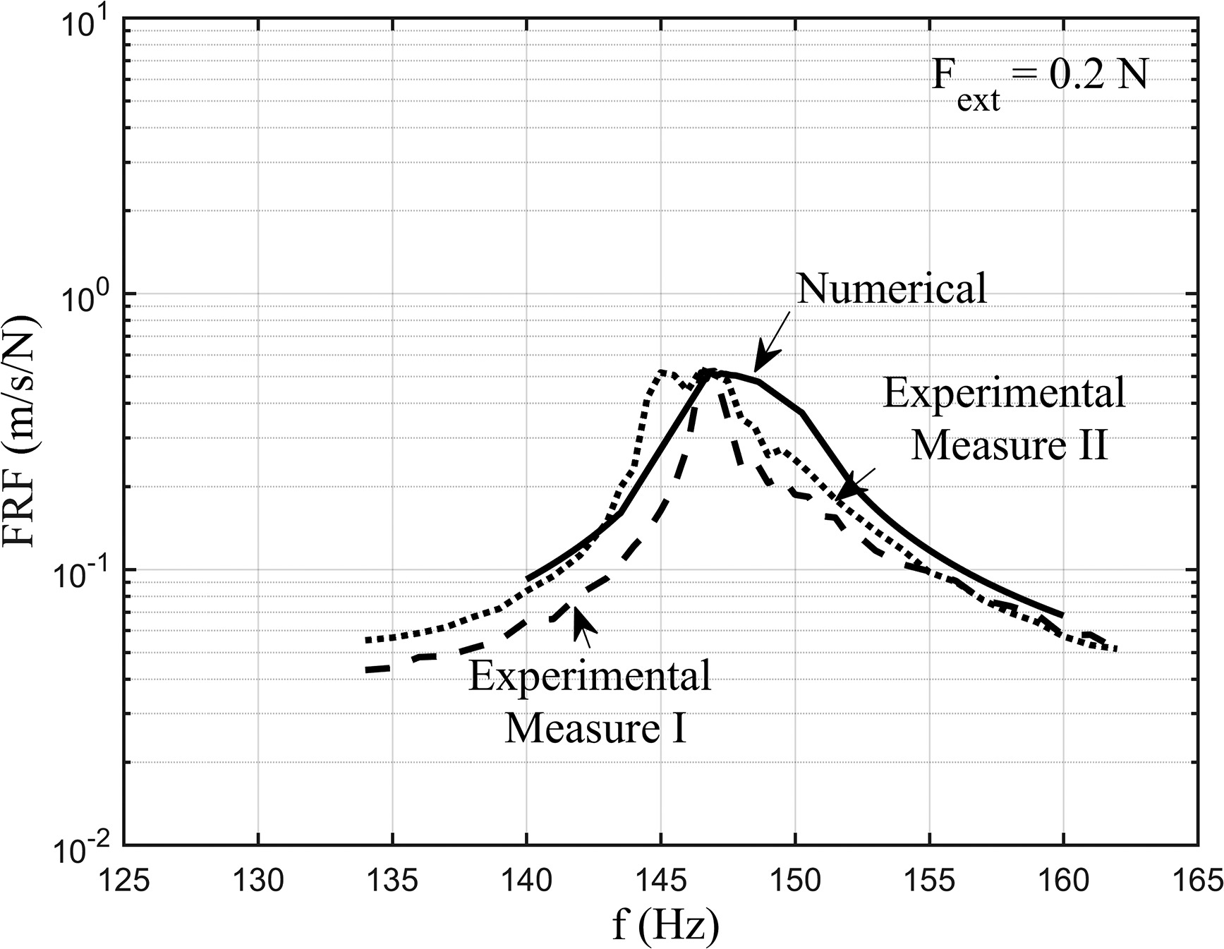
It can be observed how in this case the calculated FRFs match quite satisfactorily their experimental counterparts in terms of amplitude, shape of the peak and peak frequency. The main difference is in the value of ktx. The measured value of ktx.is one order of magnitude lower than that calculated analytically and it proves to be the correct value. The analytical method, which simulates a flat punch with a fillet radius pressed against a plane, is not fit to simulate a cylindrical contact since it gives a too high tangential contact stiffness value. This may be due to the fact that the method does not allow for micro-rotation or to the fact that it does not allow for variation of normal load. Both phenomena are instead encountered by the UPD during working condition.
Conclusions
The paper investigates two different ways to choose the contact stiffness values for the contact model of an UPDs. (1) The calculation of the contact stiffness values from the analytical models available in literature. (2) The derivation of the contact stiffness values from measurements on a dedicated test rig with a laboratory damper, but with similar working conditions of the damper under study.
The investigation is completed by the comparison of the calculated FRFs using the different values of contact stiffness with the experimental FRFs of a blisk with cylindrical UPDs. It should be noted that in this paper experimental/numerical comparison of FRFs is not used as a mean to tune the model, but as a separate and independent tool to evaluate different methods for contact parameter estimation.
Regarding the normal contact stiffness kn the analytical calculation values (Brändlein, Harris, Allara) and the value derived from measurements on the laboratory damper agree. The small discrepancies between the obtained values have negligible effects over the forced response (i.e. well below the experimental FRF dispersion).
Regarding the tangential contact stiffness ktx (in the plane perpendicular to the damper axis), Allara’s analytical method gives a value of the tangential contact stiffness ktx one order of magnitude higher than the value obtained by the derivation from measurements on the laboratory damper. In the calculation of the FRF this ktx value leads to a discrepancy >50% between the measured and simulated peak frequency. Allara’s analytical method, which simulates a flat punch with a fillet radius pressed against a plane, is clearly not fit to simulate a cylindrical contact. On the contrary the method, based on direct measurements of ktx on a dedicated test rig with a laboratory damper, produces a value of ktx one order of magnitude lower than that calculated analytically, This value of measured ktx, given to the calculation code, was successful in producing matching numerical FRFs.
In these authors opinion, the method was successful because the working conditions of the two dampers, the one tested on the dedicated test rig and the one under study, are comparable (same contact geometry, pressure, material and kinematics) and the data processing technique takes into account the difference of position and number of contact points.
These authors are therefore confident on the determination of the contact stiffness, rather than through analytical model, though careful and direct measurements on dedicated test rigs.
The results obtained here proved that measurements of contact stiffness on laboratory dampers under controlled conditions can be exported and used on other dampers.
Appendix A
It is here summarized how the values of the contact stiffness
Consider the damper equilibrium in stick condition:
where
The vector Fc in case of full stick can be expressed as:
Using transformation matrices T’ and TP’ to switch between local and global coordinate system of damper and platforms respectively:
The equilibrium can be transformed in its incremental form:
By neglecting the damper variation of inertial forces
Let us now express the variation of contact forces as a function of the variation of platform displacements by substituting in :
The last step involves isolating the horizontal and vertical components of the right contact force (HR and VR) using a transformation matrix termed here THV.
The analytical expression of entries (1,1) and (1,3) of matrix
is unique and allows determining kn and ktx. The values thus obtained are then normalized by the length of contact of the three point damper and multiplied by L, the length of contact of the cylindrical damper. The stiffness for each contact point can then be determined by dividing the obtained values by the number of the chosen contact points.