Nomenclature
β:
rotation
CF:
centrifugal force on the damper
H:
horizontal force on the damper
k:
contact stiffness
µ:
friction coefficient
N:
normal force on the damper
n:
normal displacement
θ:
platform angle
T:
tangential force on the damper
t:
tangential displacement
u:
horizontal displacement
V:
vertical force on the damper
w:
vertical displacement
Introduction
Friction damping devices are commonly used in turbines to reduce the vibration amplitude of blades in resonant conditions (02). One of these devices is the underplatform damper (UPD). The UPD is a small, cheap, metal component positioned at the underside of two adjacent blades (22). UPDs can come in different shapes (cylindrical, wedge or asymmetrical) (01). As already pointed out in (17, 19) the asymmetrical configuration is preferred since, unlike cylindrical dampers, it avoids rolling (loss of stiffness and lower dissipation) and, unlike wedge dampers, it self-adapts its position and the contact with the platforms is ensured even for large platform displacements.
The presence of UPDs serves a double purpose: (1) it introduces additional mass and stiffness, thus shifting the resonance frequency of the damper-blades system (2) the relative motion between the damper and the platforms causes energy dissipation through friction, thus introducing additional damping.
Nevertheless, the UPD contribution to stiffness and damping is not easy to predict. To this purpose, a complex hierarchy of numerical techniques has been developed in the last two decades (18, 05, 19, 06, 07, 21). However, whatever the numerical technique, a solution simultaneously correct for the damper and the blade dynamics is found if and only if their interface forces are correctly reproduced.
Trustworthy predictions of contact forces are largely dependent on the appropriate choice of contact parameters (i.e. friction coefficients and contact stiffness values), as demonstrated in (20). The need for the safe determination of contact parameters led to AERMEC’s Test Rigs. Some focus on single contacts under constant normal loads and high temperatures (16, 03, 15), while the Damper Test Rig, built in 2008 (10) aims at estimating contact parameters of UPDs under more realistic working conditions in terms of variable normal load and complex interface kinematics. Since then, the test rig has been used to investigate the behaviour of several dampers in terms of kinematics and force transmission characteristics (13). Subsequent improvements have been performed on the test rig structure, to increase its operating frequency range (11) (now up to 160 Hz) and the contact pressure on the damper (08) (up to 6 MPa for plane-on-plane contacts).
A numerical model of the damper/test-rig system was first presented in (13), together with the first version of the contact parameters estimation procedure. This first procedure was successful in estimating friction coefficients, however the contact stiffness problem was left under-determined.
The first section of the paper overcomes this limitation, thus identifying a unique value for each of the four contact stiffness — left and right damper-platform contact, normal and tangential. In it, new experimental capabilities and data processing techniques are added to the measurement protocol developed by these authors in (13). Specifically, platform-to-damper measurements of tangential force vs. relative tangential displacement (platform-to-damper hysteresis cycles), left and right, first presented in (09) are here improved and analysed. Tangential contact stiffness values are directly the slopes of those hysteresis segments which are safely identified as being in a stick condition. In flat-on-flat contacts which are often found in solid dampers, normal contact stiffness values cannot be measured directly. This paper proposes to deduce them by plotting the damper-platform relative rotation vs. the contact force eccentricity, introducing a novel formulation which overcomes the limitations found in (09). By these means all contact parameters are determined for a solid damper purposely designed to avoid undesirable lift-off and to allow accurate experimental conditions (08).
Uncertainty estimates are also shown. The section is closed by feeding the contact parameters into a numerical model representing the damper in the test rig including the rig’s own pertinent spring values: on this basis, a numerically simulated platform-to-platform cycle is compared against its experimental counterpart.
The second section of the paper numerically investigates the influence of variations of each damper-to-platform contact parameters on those platform-to-platform blade coupling factors which are of a major relevance to engineering applications. The following have been chosen: the real and the imaginary parts of the coupling stiffness, i.e. the equivalent spring and damping values. The sensitivity of each contact parameter can thus be compared against its experimental accuracy from the first section.
The test rig
The test rig (see Figure 1), developed over the years by the AERMEC laboratory, is designed aiming at:
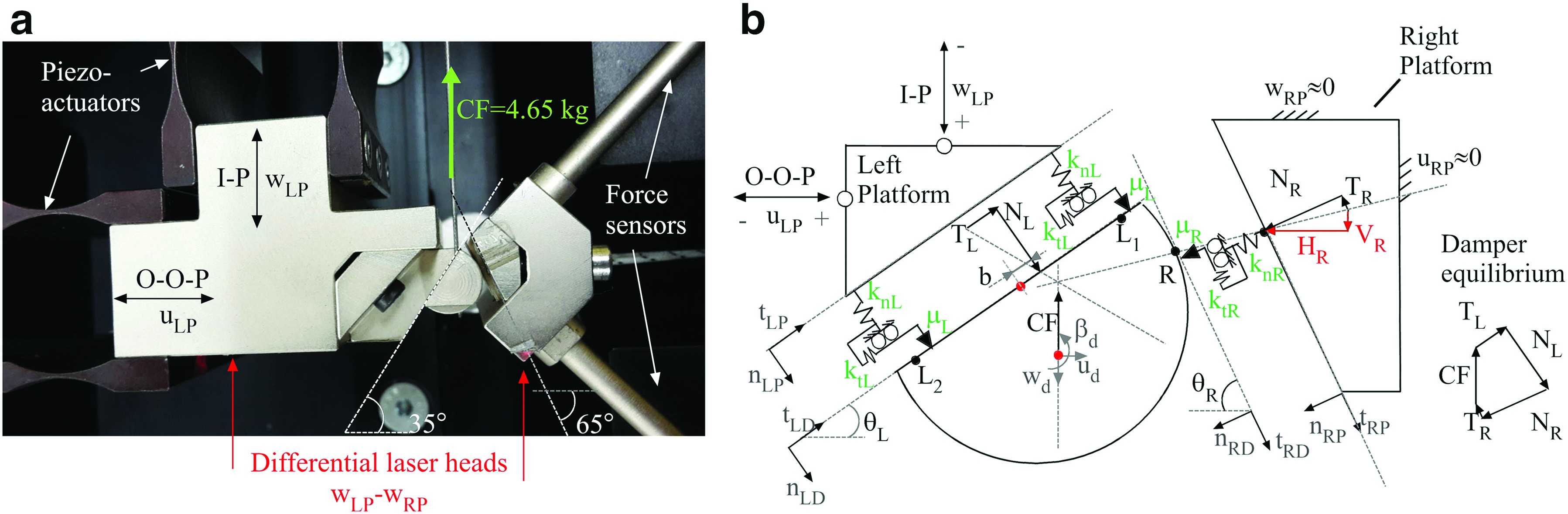
imposing user-defined in-plane harmonic displacements simulating the so-called In-Phase (vertical) and Out-of-Phase (horizontal) relative motion between the blades platforms or combinations of the two;
measuring the forces transmitted between the two platforms through the damper;
measuring the damper in-plane kinematics.
To achieve the first goal the left platform is connected to two piezoelectric actuators. To achieve the second goal the right platform is connected to two uniaxial force sensors by means of a tripod and the damper is pulled by a deadweight simulating the centrifugal force. The third goal is achieved by utilizing a differential laser head to measure the platforms relative displacement (a necessary precaution owing to the lack of closed loop control of the piezoelectric actuators) and the damper radial displacement and rotation angle. A complete description of the test rig and of the measurement protocol can be found in (13).
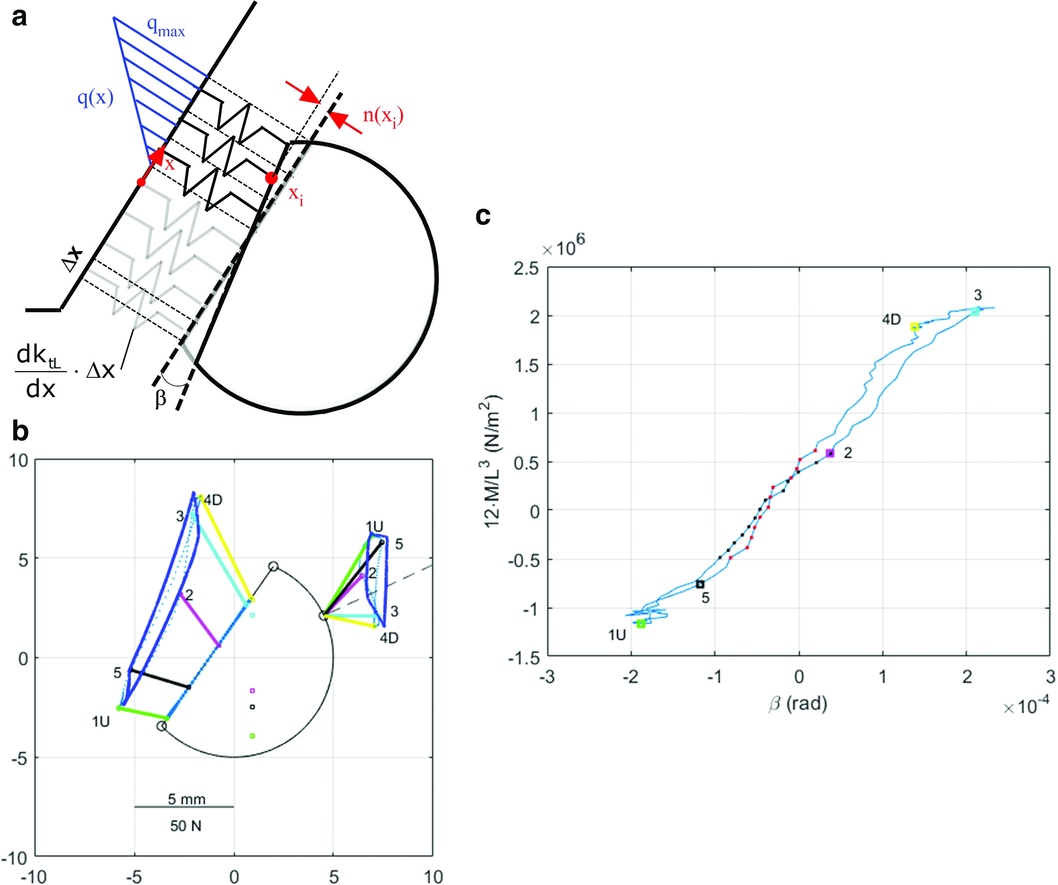
The ultimate goal of the test rig is to relate the imposed displacement (1) to the contact forces (2) in order to record the damper platform-to-platform hysteresis loop (as shown in Figure 2) and link its different portions to the corresponding damper kinematic behaviour (3). The area of the global hysteresis cycle represents the energy dissipated by the damper.
Figure 2.
Measured (dotted line) and simulated (solid line) platform-to-platform IP cycle for the damper in Figure 1.

The numerical model
Figure 1 shows the numerical model of the damper/platform system. In it, the damper is modelled as a rigid body with mass and inertia properties. The rigid body assumption is considered valid given the bulkiness of the damper and has been successfully applied to several test cases in the last few years (12, 13, 08). The relative motion imposed to the platforms is harmonic to simulate the motion of the blades at resonance (and that of the test rig).
The contact model used is a standard macroslip element (22). The following section will present the procedure used to tune the contact parameters (six in total): with reference to Figure 1 friction coefficients (
The benchmark case
The chosen experimental benchmark has been obtained by imposing a 5 Hz, wLP = 30 µm (reduced to 22 µm due to the lack of a closed loop control on the piezo) In-Phase harmonic motion to the left platform. The centrifugal load on the damper is set at 50 N. The frequency is set to 5 Hz in order to have a quasi-static hysteresis measurement (i.e. cleaner signal) for contact parameter estimation. It should be noted that the damper has been tested in the complete frequency range allowed by the test rig ([5–160 Hz]) and the results have been found unchanged, as already shown in (11).
The centrifugal force is set at 50 N. However, the contact pressure is greatly increased by the presence of two 4 mm long tracks on the platforms, described in (08) and partially visible in Figure 1. These tracks have a double function: they standardize the length of contact and increase the contact pressure to 50% of that experienced by a 170 mm long damper with the same cross section mounted on the fourth stage of a turbine for energy production.
Figure 2 plots the comparison between numerical and experimental vertical platform-to-platform hysteresis cycle. The measured cycle is reproduced very satisfactorily (error on equivalent stiffness and damping <1%). Moreover, it should be noted that this piece of experimental evidence was not used during tuning.
Figure 3 to Figure 5 display additional experimental diagrams, relative to the same measurement and experimental conditions: this set of diagrams, described in the following section will be used to estimate the damper/platforms contact parameters.
Estimation of contact parameters
The following paragraphs describe the estimation procedure for each of the six contact parameters needed to calibrate the damper model. For each contact parameter a subsection is devoted to estimation accuracy. In all cases the authors have taken into account three contributions: measurement uncertainty (due to instruments uncertainty, properly propagated where needed), uncertainty introduced by data processing techniques (e.g. reading error) and finally sample-to-sample variability (if the measurement is repeated the result may change). Depending on the specific contact parameter, one or more contributions may be negligible with respect to others.
Friction coefficients
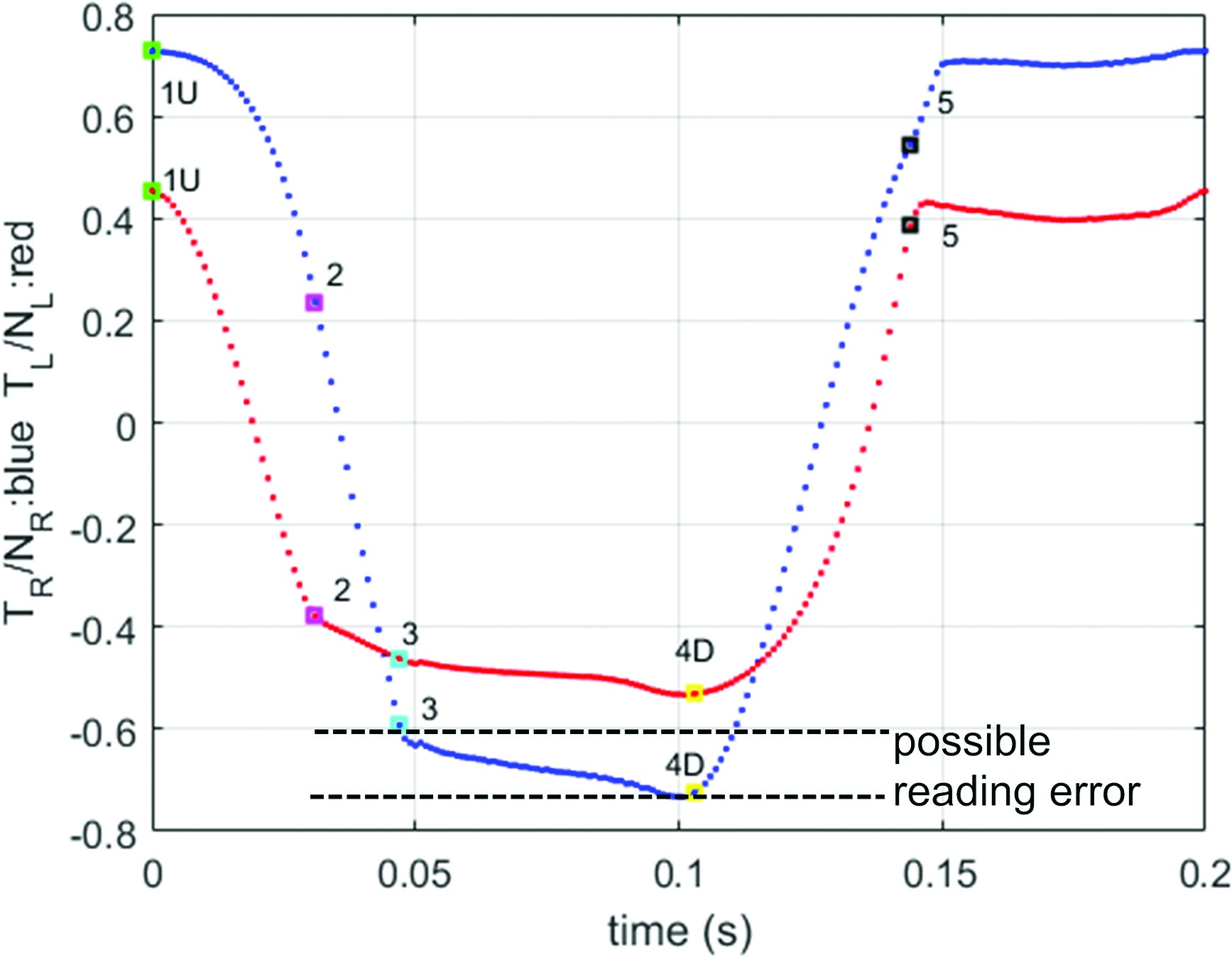
Friction coefficients at both interfaces are estimated using the time history of the tangential/normal force ratio at the two contacts as described in (13, 08). If the force ratio is constant in time and equal to a maximum then it is assumed to be a friction coefficient (e.g. 3-4D and 5-1U in Figure 3). The measured values for the case in Figure 3 are reported in Table 1.
Table 1.
Accuracy and limits to ensure a 5% error on KR and KI for friction coefficients
| Parameter | ||
|---|---|---|
| Nominal value | 0.7 | 0.45 |
| Experimental accuracy | [0.62–0.78] | [0.38–0.52] |
| Limits to ensure | [0.65–0.75] | [0.21–0.57] |
| Limits to ensure | [0.61–0.78] | [0.31–0.54] |
The components of the right contact force (TR and NR) are directly measured, while the left components (TL and NL) are reconstructed: the numerical model has shown that inertia effects of the damper are negligible in the investigated frequency range therefore it is possible to reconstruct the equilibrium as shown in Figure 1.
Estimation accuracy
The variability between independent measurements is negligible, therefore the estimation accuracy includes two effects: the uncertainty on the force components (4% on TR/NR and 8% on TL/NL) derived from the load cells specifications and from subsequent error propagation techniques (13) and the error committed in reading the value on the diagram (≈±0.05 as shown in Figure 3). These two effects are summed is a maximizing indicator (i.e. the actual error will be certainly contained within those limits), shown as an error bar in Figure 8.
Figure 8.
Friction coefficient

The variation of the T/N force ratio during slip is slightly sharper in the case of the right contact (cylinder-on-flat), possibly due to the different interface and the different platform angles. This behaviour is quite repeatable and may indicate that a contact model with constant friction coefficient is not completely adequate to represent reality (i.e. the authors have willingly turned epistemic uncertainty into measurement uncertainty). However, as it will be shown later the effect of this variation produces negligible effects on the output quantities of interest at blade level, therefore these authors still deem the model adequate.
Tangential contact stiffness values
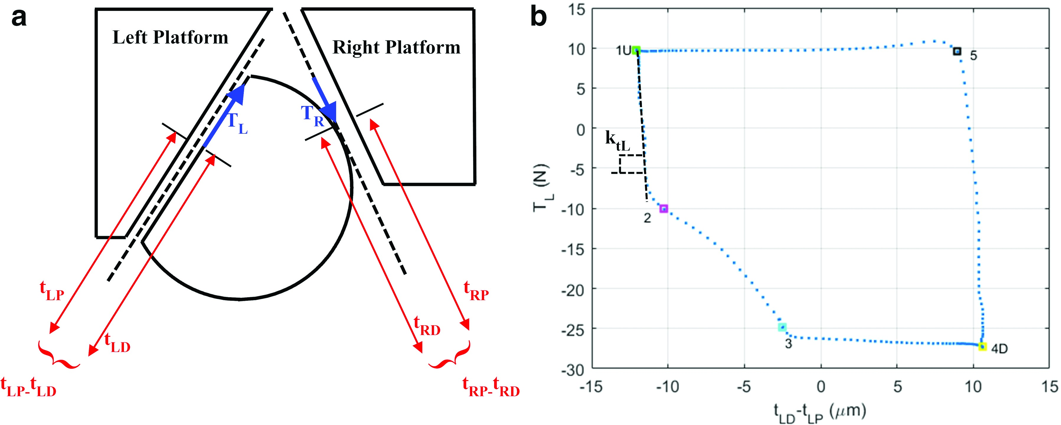
The dummy platform have been recently equipped with cube-like protrusions oriented with one of the faces perpendicular to the contact line (see Figure 4). Each contact line (left and right) is equipped with two cubes (one on the damper and one on the corresponding platform). This allows for the measurement of the tangential relative motion at the contact. The hysteresis at the contact (as shown in Figure 4) is obtained by relating this relative motion to the corresponding tangential force: the slopes of the portion of hysteresis cycle identified as being in stick condition can be used to estimate the tangential contact stiffness values on each side of the damper. The stick condition is identified by looking at the corresponding T/N force ratio in Figure 3 (e.g. stage 1U-2 is identified as stick because TL/NL is not constant in time) as shown in (09). Cylinder-on-flat and flat-on-flat contact interfaces have both been tested.
Figure 4.
(a) Functional scheme representing the experimental procedure used to estimate the tangential contact stiffness values. (b) Measured platform-to-damper hysteresis at the left contact.
Estimation accuracy
In this case measurement uncertainty (13, 09) (error on dynamic variation of force summed to error on laser recorded displacement) is one order of magnitude lower with respect to the uncertainty introduced by the data processing technique. In fact, results change slightly depending on the portion of curve identified as being in stick condition. Therefore, the accuracy is here assessed by repeating the procedure on five independent measurements and thus computing the standard deviation. This technique ensures that uncertainty caused by sample-to-sample variability is taken into account as well. The results are reported in Table 2.
Table 2.
Accuracy and limits to ensure a 5% error on KR and KI for tangential contact stiffness ktR, ktL.
Flat-on-flat normal contact stiffness
The normal contact stiffness at the flat side knL is assumed to be uniformly distributed along the flat interface, dknL/dx (see Figure 5, 09). As shown in Figure 5 during the cycle the normal component of the left contact force resultant NL travels along the flat surface during the cycle. If NL enters the inner third portion of the flat interface, then the complete surface is in contact. Under this condition, it is possible to write the moment of NL around O (see Figure 5) as a function of the rotation β:
The normal contact stiffness per unit length is the slope highlighted in Figure 5. It should be noted that the slope has been estimated using a specific portion of the curve in Figure 5: the portion corresponds to instants in the cycle where NL falls inside the inner third portion of the contact interface. This can be estimated checking the corresponding experimental diagram in Figure 5.
Estimation accuracy
In this case measurement uncertainty (derived from instruments specs and error propagation techniques) is one order of magnitude lower with respect to the uncertainty introduced by the data processing technique. In fact, results change slightly depending on the selected portion of curve. Therefore, the accuracy is here assessed by repeating the procedure on five independent measurements and thus computing the standard deviation. This technique ensures that also uncertainty caused by sample-to-sample variability is taken into account. The results are reported in Table 3.
Cylinder-on-flat normal contact stiffness
The normal contact stiffness for the cylinder-on-plane contact has been obtained by taking the initial slope of the corresponding normal displacement-normal force curve. This curve has been obtained from interpolations of experimental data (14), later confirmed by theoretical investigations (04).
Estimation accuracy
The value depends on the length of contact, which depends on machining tolerance (see Table 3). However, that source of uncertainty has negligible effects. The real source of uncertainty comes from the model itself (epistemic uncertainty), which may not be representative of an evolving and potentially worn contact. Thankfully it will be shown in the following sections that moderate variations of the normal contact stiffness have negligible effects (<5%) on the equivalent stiffness and damping introduced by the damper.
Results and discussion
Harmonic complex springs: equivalent stiffness and damping
The nonlinear dynamic response is usually computed using Harmonic Balance methods (HBM) where forces and displacements are decomposed in their harmonic components. If the platforms’ imposed displacement is assumed to be mono-harmonic
Figure 6.
Hysteresis cycle with imposed displacement
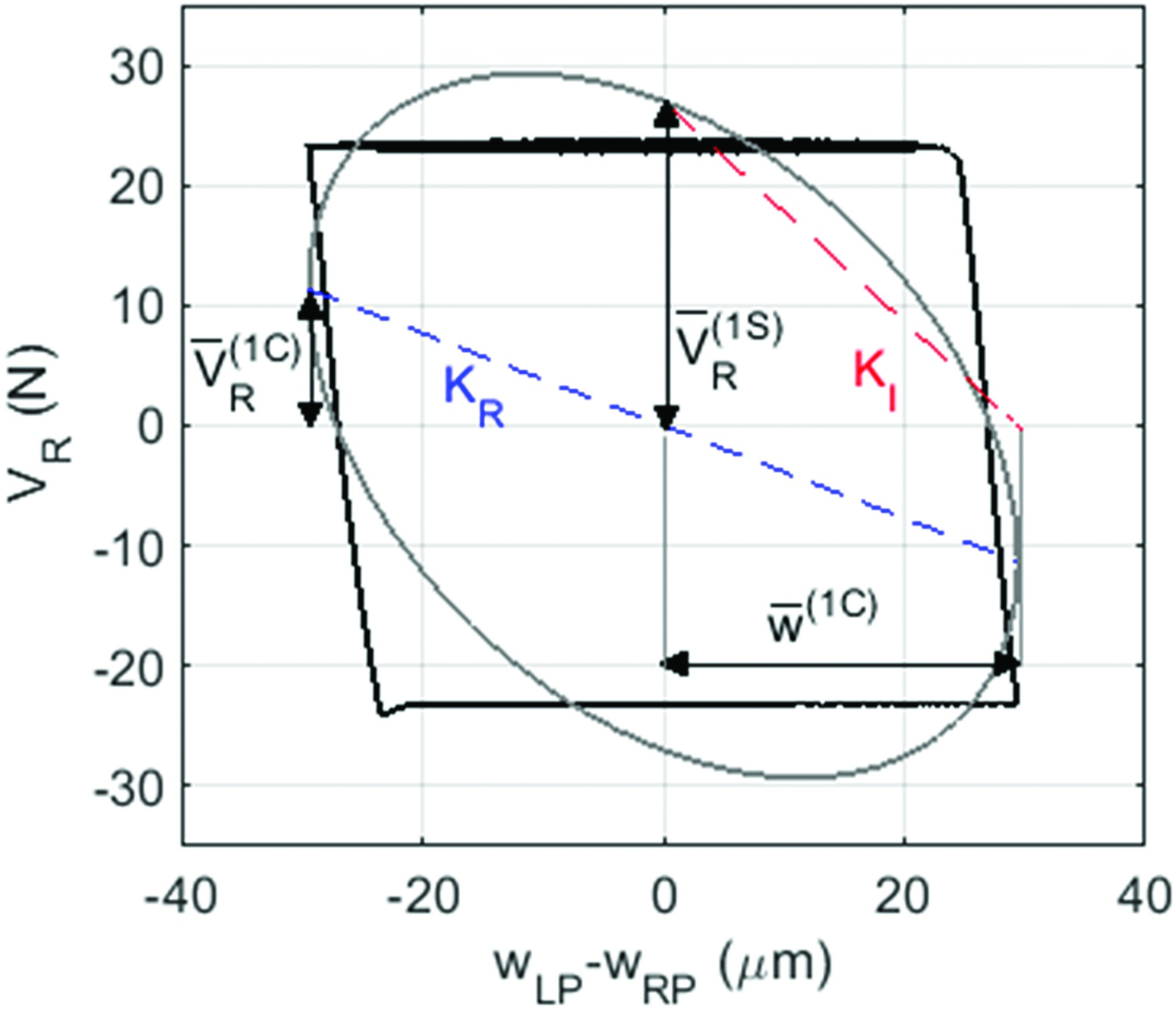
Figure 7 plots the complex springs values against the imposed displacement

Sensitivity
The purpose of this section is to show the acceptable variation of each contact parameter to ensure an error on the performance indicators limited to 5%
This numerical analysis is carried out for platforms’ imposed displacements ranging from
Sensitivity to variation of friction coefficients
Figure 8 plots the acceptable variation of the friction coefficient on the cylindrical side (
In Figure 8 the black dashed line corresponds to the value of friction coefficient estimated using the procedure presented in the previous section and is assumed to be the correct one. The corresponding error bars are located at
Several caveats can be drawn from the observation of these diagrams:
in the
in the
generally speaking an increase of friction coefficient produces an increase of the dissipated energy (
when platforms’ displacement is limited (in the range of
as evidenced in Table 1 the accuracy obtained with AERMEC’s estimation procedure allows for a safe prediction of the equivalent spring values.

Sensitivity to variation of contact stiffness values
Figure 10 plots the acceptable variation of the tangential contact stiffness at the flat side (
Figure 10.
Tangential contact stiffness ktL acceptable variation to ensure an error on the performance indicators limited to 5%
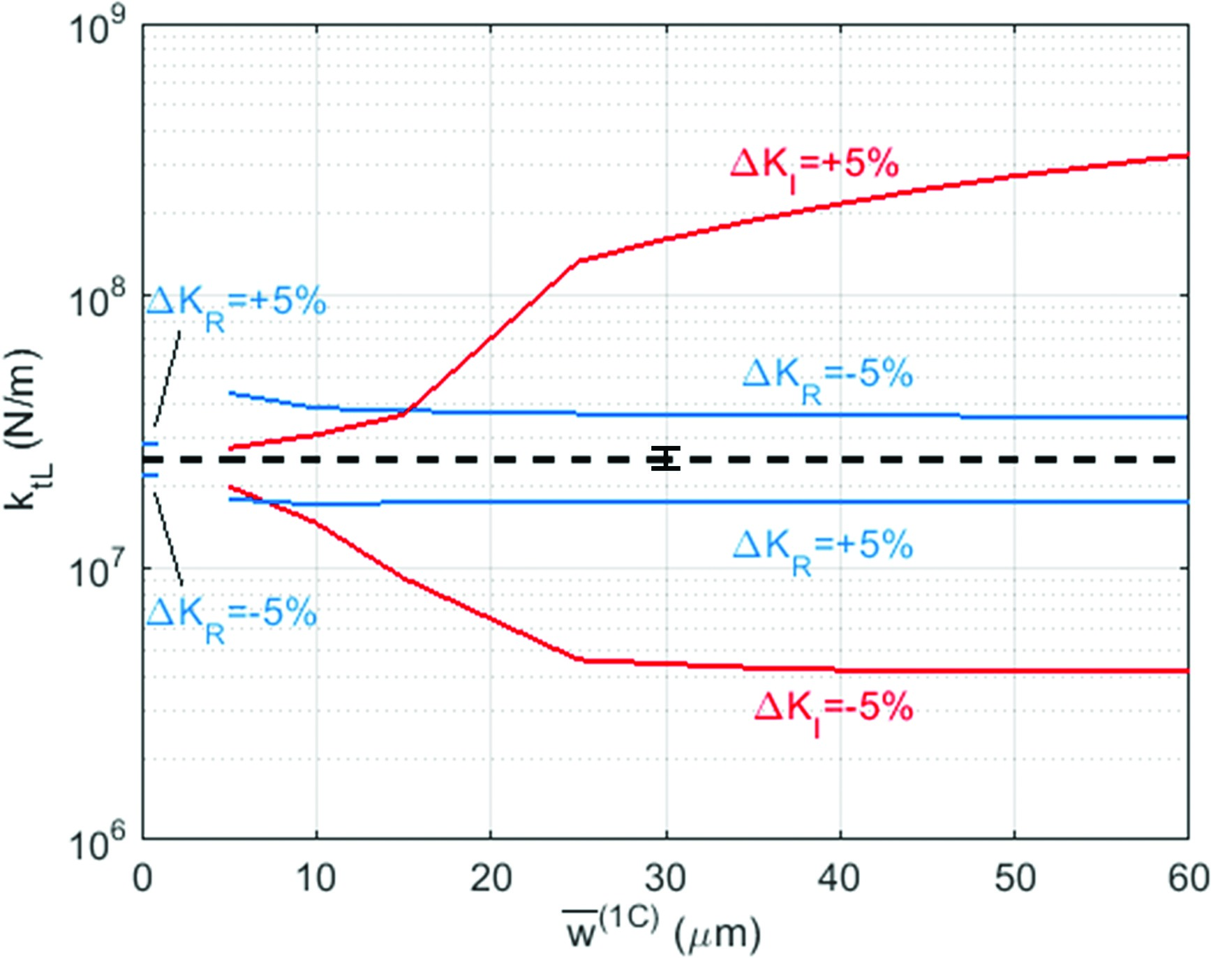
In Figure 10 the black dashed line corresponds to the value of contact stiffness estimated using the procedure presented in the previous section and is assumed to be the correct one. The corresponding error bars are located at
Several caveats can be drawn from the observation of these diagrams:
in the
in the gross slip range
in the
in the range
in the gross slip range
as evidenced in Table 2 and Table 3 the accuracy obtained on the tangential contact stiffness values is comparable with the |ΔKR| and |ΔKI| 5% limits.
as evidenced in Table 3, knR, being the highest, has a very low influence compared to the others.
Conclusions
The paper presents an extension of the existing contact parameter estimation technique, first described in (13). Specifically, a new set of experimental evidence (hysteresis cycles at the contacts and moment vs rotation diagram) was used to uniquely estimate the contact stiffness values. The contact parameters thus obtained have been fed to the numerical routine, which successfully represented the platform-to-platform hysteresis cycle.
This set of contact parameters served as a reference point to conduct a sensitivity analysis. The real and the imaginary parts of the platform-platform coupling stiffness, (i.e. the equivalent spring and damping values) have been chosen as output indicators (blade-level).
The numerical analysis has shown that the proposed contact parameters estimation technique, entirely based on direct measurements on dampers, ensures an uncertainty on the output indicators in the 5% range.