
Introduction
Rotating machinery is the key equipment which is widely used in aviation, ship, electric power and other fields. As the core component of rotating machinery, blades are directly related to the safety of the equipment. Blades are easy to vibrate because they usually work under harsh conditions for a long time (Abdelrhman et al., 2014). The most common flow-induced vibration is due to rotor-stator interaction (Zhao et al., 2019). However, blade vibration is one of the main reasons which may lead to serious work failure (Carter, 2005). The unsteady aerodynamic load is inherent and can cause large amplitude blade vibration and even high cycle fatigue (HCF) failure (Zhao et al., 2019). Therefore, it is crucial to monitor the vibrations of blades, especially large amplitude vibration. Blade tip timing (BTT) is a powerful means of non-contact online measurement of blade vibrations. Compared to the conventional strain gauges (SGs), BTT has some outstanding advantages such as being capable of long-time online monitoring of all the blades in a row and easy to deploy (Knappett and Garcia, 2008). These advantages make BTT get more popular in the field of blade testing and monitoring of rotating machinery.
The basic process of measuring by BTT technology is first installing several BTT sensors on the fixed casing and acquiring the actual arrival time to sensors’ circumferential installation positions with existences of blade vibrations. Then we can get the ideal arrival time without blade vibrations and obtain the blade tip displacements by calculating the differences between the actual arrival time and the ideal arrival time (Russhard, 2010). The number of BTT sensors installed is limited on a casing in actual measurements, and it is likely that the rotational frequencies are much lower than the natural frequencies of blades. The sampling frequency equals to the rotational frequency multiplied by the number of BTT sensors installed. According to the sampling theorem, BTT signals are probably under-sampled. Corresponding identification and reconstruction algorithms are needed to extract effective information from original data (Chen et al., 2021).
Synchronous vibration is a common vibration form of blades of rotating machinery. The vibration frequencies of blades are integral multiples of the rotational frequencies (Carrington, 2002). The displacement data collected by a BTT sensor is the same in every sampling cycle at the resonance rotational speed, so it is difficult to identify the parameters of synchronous vibration. The identification algorithms for synchronous vibration currently include Zablotsky-Korostelev Single Parameter Technique (SPT/traditional SPT) (Zablotsky and Korostelev, 1970), Two-Parameter Plot Method (Heath, 2000), Autoregressive Method (Dimitriadis et al., 2002), Circumferential Fourier Fit (CFF) method (Joung et al., 2006) and so on. In these methods mentioned above, SPT is widely used because of the low demand for circumferential installation positions and number of BTT sensors. SPT changes the frequency of excitation force passing through the resonance area of blade by changing the rotational frequency and obtains the curve of the blade tip displacement vs rotational speed to identify the parameters of vibration. But this method assumes that the influence of blade’s own vibration on arrival time can be neglected. Ignoring the influence of blade’s own vibration on arrival time and directly using the circumferential installation positions of the BTT sensors will result in errors in parameter identifications. If we use this method to identify vibrations of rotating blades with large amplitudes, there would be errors in identifying maximum vibration amplitude because of the above-mentioned assumption. Heath and Imregun (1996, 1997) raised this problem in former researches, but they only simply analyzed the existence of the errors by a numerical simulator and did not study in depth. Therefore, it’s essential to revise the traditional SPT to reduce the errors in identifying the parameters of vibrations with large amplitudes related to BTT actual measurement and analyze the sources and characteristics of the errors parametrically.
In this paper, a revised method for both large and small amplitude vibration parameter identification related to BTT actual measurement based on single degree of freedom (SDOF) blade model is proposed. The accuracies of the revised method and traditional SPT for identifying the maximum vibration amplitude are compared by numerical experiment. The main source of the error and the error characteristics caused by fitting according to traditional SPT are also analyzed. An experimental bench is used to verify the revised measurement formula. The third section shows a new revised mathematical model of single degree of freedom(SDOF) blade model discarding the assumption of small amplitude related to BTT actual measurement and its derivation process. The fourth section explores the sources and characteristics of the errors in identify the parameters of vibrations with large amplitudes by numerical experiments when using traditional SPT and analyzes the accuracy of the revised method. This section also introduces the experimental platform and its parameters, as well as verifies the correctness of the revised method. The fifth section summarizes the results of the study.
Methodology
Consider that the blade is a vibrational system with single mode, SDOF, damping and a constant-amplitude harmonic excitation force. This vibrational system can be described by this equation (Zablotsky and Korostelev, 1970):
where y is the dynamic blade tip displacement; ζ is the damping ratio; ω0 is the natural angular frequency of blade; F0 is the amplitude of excitation force; m is the mass; ω is the angular frequency of excitation force; φ0 is the initial phase.
The steady-state solution of the above vibration equation is:
where
ycm is the static shifting of blade tip under the action of force F0, i.e., ycm = F0/(mω02). The meanings of terms in Equations (3) and (4) are the same as those in Equation (1).
For the vibration due to forced response, the frequency of excitation force is closely related to the rotational speed (Cumpsty and Greitzer, 2004). When the rotor is operating at a constant rotational speed, the frequency of excitation force can be regarded as a constant number. By assuming that the excitation force is dominated by single engine order, the frequency of excitation force can be expressed as:
where k is the engine order; Ω is the rotational speed (Unit is rad/s).
Using BTT technology to measure the blade tip displacement, the expression of measured blade tip displacement is (Xiao et al., 2022):
where tni is the time that the ith blade triggers the only BTT sensor in the nth revolution; ϕ(tni) is the angular displacement of the rotor at time tni;
The angular displacement of the rotor ϕ(t) can be written as:
where tkey,n is the time when the keyphasor sensor is triggered at the beginning of the nth revolution.
When the rotational speed is constant, the angular displacement of the rotor ϕ(tni) at time tni can be represented as (Heath and Imregun, 1996):
Let
We can get:
The corresponding dynamic blade tip displacement yni at time tni is:
We can combine Equations (10) and (11):
For synchronous vibration, k is an integer. So we can get:
Equation (13) takes the influence of blade’s own vibration on arrival time into consideration and discards the assumption of small amplitude. This new revised method can apply to both small amplitude and large amplitude. It should be emphasized that because k is multiplied by the term
The measured blade tip displacement xni is effected by many factors, including existence of multi-modal response, steady offsets (Xiao et al., 2023) and the stagger angle of the blade. Therefore, the measured blade tip displacement is not equivalent to the dynamic blade tip displacement yni. The dynamic blade tip displacement should be a function of measured blade tip displacement:
where
We can get:
The actual arrival time tni of Equation (11) also contains two parts. One is due to the blade rotation, the other is due to the blade’s own vibration. Traditional SPT neglects the influence of blade’s own vibration on arrival time (the second part) and directly uses the circumferential installation positions of the BTT sensors (Heath and Imregun, 1997). In addition, measured blade tip displacements are probably wrongly used to identify parameters as dynamic blade tip displacements when using traditional SPT (Chen et al., 2021):
The first problem of Equation (16) is wrongly using xni as the left term. Moreover, term
Assume a straight blade with only single-modal response and none steady offset in rotation. The direction of blade vibration and the detection direction of BTT sensor are the same. The measured blade tip displacement has no errors and no noise. We can obtain:
Under this circumstance, Equations (13) and (15) can be written as:
Results and discussion
Numerical experiment
Consider a simple straight aluminum alloy blade. Its first bending vibration can be equivalent to a SDOF spring-damper vibration model. To simplify the numerical experiment, let the steady offset in rotation be zero. The preconditions of Equation (17) are all satisfied. According to the result of Campbell diagram, it was found that when the rotational speed was 656 rpm, the external force due to the excitation led to synchronous vibration with k = 5.0. At this time, its first natural frequency is about 54.67 Hz (Tian et al., 2022). The parameters of this case are listed as following. The blade tip radius r is 0.27 m. Given ycm = 0.0002 m,
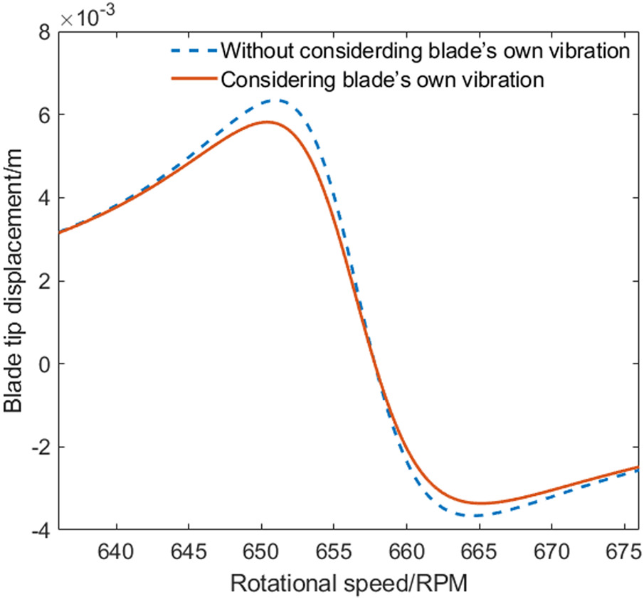
Figure 1.
Comparison between the blade tip displacement obtained by considering the influence of blade’s own vibration on arrival time and not.
For the above-mentioned blade, the error between the maximum vibration amplitude Amax obtained by fitting according to Equation (16)/[Equations (13) or (18)] and the given real maximum vibration amplitude is studied by the control variable method when only changing ycm, ζ,
where
Figure 2.
The error between the maximum vibration amplitude obtained by fitting according to traditional SPT and the given real maximum vibration amplitude. (a) ycm-Error Curve (b) ζ-Error Curve (c) θ ¯ ¯ i
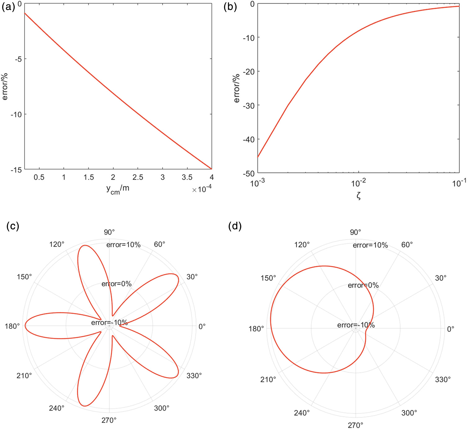
Figure 2 shows the error between the maximum vibration amplitude Amax obtained by fitting according to traditional SPT [Equation (16)] without noise and the given real maximum vibration amplitude. It can be seen from Figure 2(a) that when ycm (i.e., the amplitude of excitation force) increases, the error between the maximum vibration amplitude obtained by fitting and the real value is also larger, and the relationship between ycm and the error is almost linear. The reason is that when the amplitude of excitation force increases, the vibration amplitude of blade will also increase. When ycm is larger, the influence of blade’s own vibration on arrival time becomes more and more significant and cannot be ignored.
From Figure 2(b) it can be seen that when the damping ratio ζ decreases, the error between the maximum vibration amplitude obtained by fitting and the real value is greater, and when the damping ratio is relatively small, the error increases rapidly to a large number, indicating that when the damping ratio is small, the error is very sensitive to the change of damping ratio. This is mainly due to the increment of vibration amplitude. We should not only use the installation position of sensor in the fitting.
Figure 2(c) shows that when
It can be seen from Figure 2(d) that when the initial phase φ0 changes, the changing trend of error between the maximum vibration amplitude obtained by fitting and the real value is similar to that in a period when
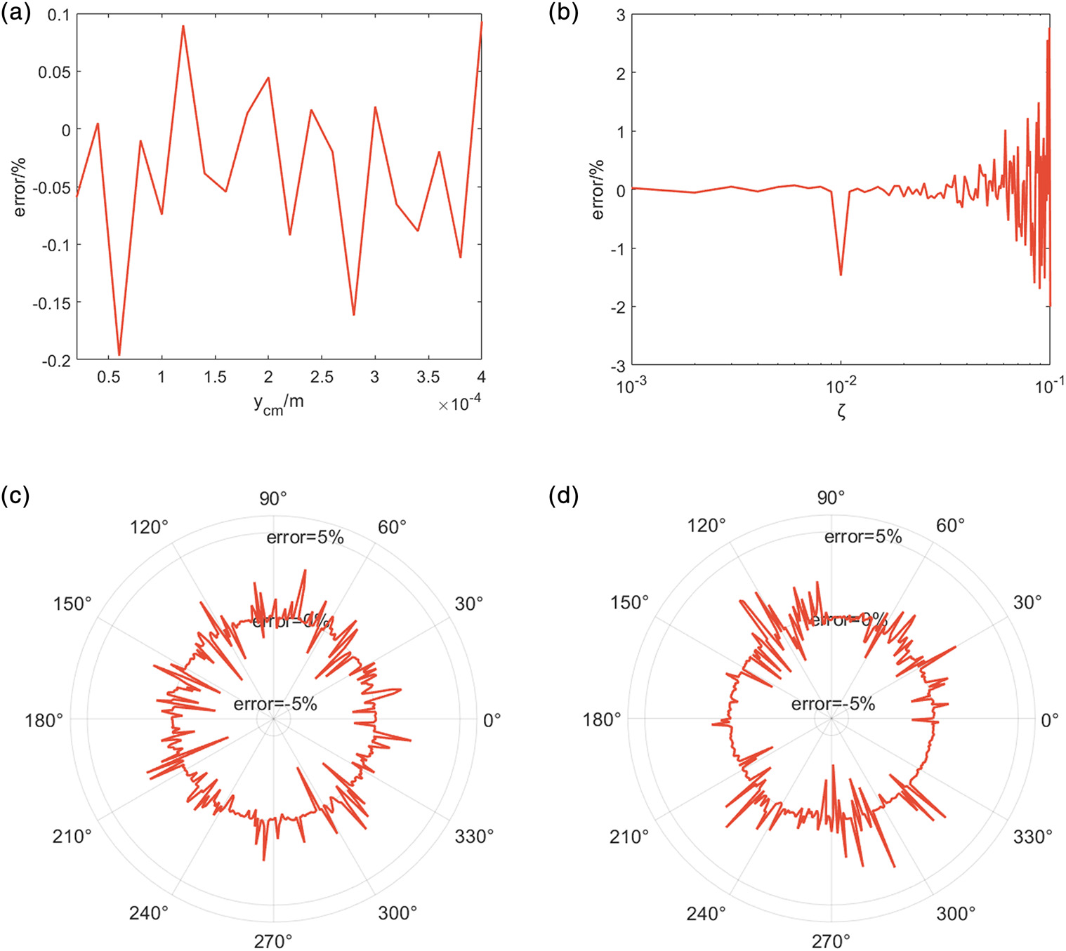
Figure 3 shows the error between the maximum vibration amplitude Amax obtained by fitting according to the new revised method [Equations (13) or (18)] and the given real maximum vibration amplitude (The initial conditions of each parameter and fitting options in this fitting are the same as those in Figure 2). The preconditions of Equation (17) are all satisfied, except for no noise. The signal-to-noise ratio (SNR) is 40 dB. It can be seen from Figure 3 that when the four factors are changed respectively, the error between the maximum vibration amplitude obtained by fitting and the real value is reduced to a small value. Under the above conditions, almost all the errors are less than 3%. This indicates that there are quite small errors between the fitting values and the real values, and the accuracy of vibration parameter identification is greatly improved, which proves the validity of the new revised method.
Figure 3.
The error between the maximum vibration amplitude obtained by fitting according to the new revised method and the given real maximum vibration amplitude (SNR = 40 dB). (a) ycm-Error Curve (b) ζ-Error Curve (c) θ ¯ ¯ i
The error caused by fitting according to traditional SPT [Equation (16)] was further studied, and the object is still the simple straight aluminum alloy blade mentioned above. The errors between the vibration parameters obtained by fitting and the given real parameters in different cases were compared. Table 1 shows the given parameters in different cases. Table 2 shows the errors between the vibration parameters obtained by fitting and the given real parameters. Δφ0 is the difference between the initial phase obtained by fitting and the real initial phase, others show the percentage of errors between the vibration parameters obtained by fitting and the given real parameters.
Table 1.
The given real parameters in different cases.
Table 2.
The errors between the vibration parameters obtained by fitting and the given parameters.
It can be seen from Table 2 that the biggest problem of the parameters obtained by traditional SPT appears in the damping ratio ζ term. The relatively large error basically appears in the damping ratio term, and the errors of other parameters, such as ycm, ω0 and k, are very small. The error of Amax is also mainly due to the error of damping ratio. Therefore, the accurate identification of damping ratio is very important in the experiment, which will directly affect the accuracy of the vibration identification. The parameters ycm, ω0 and k fitted by traditional SPT have relatively high accuracies, so traditional SPT can be used to identify these three parameters. But the revised method is still needed to accurately identify the damping ratio.
We changed the research object to a fan blade and continued to study the error characteristics caused by fitting according to traditional SPT. It was found that when the rotational speed was 1,770 rpm, the external force due to the excitation led to synchronous vibration with k = 2.0. At this time, the first natural frequency of the blade is about 59 Hz. The parameters of this case are listed as following. The fan blade tip radius r is 0.98 m.
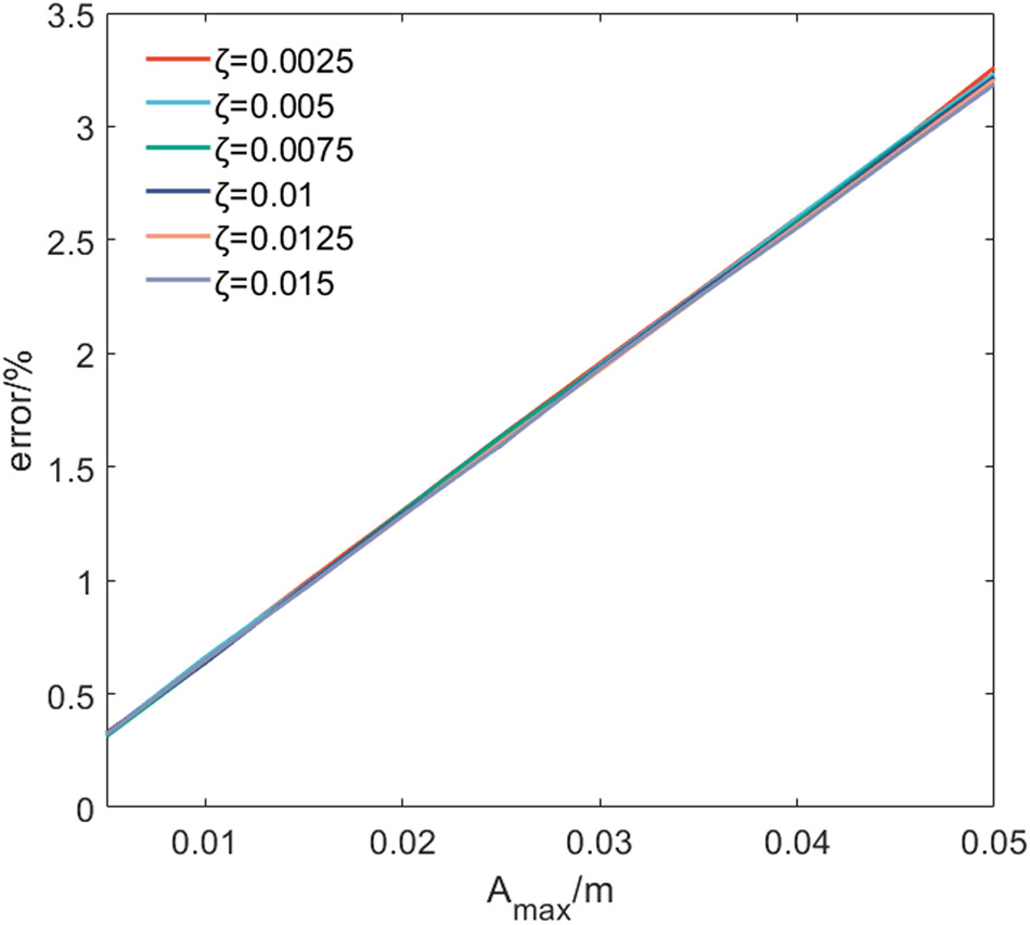
Figure 5 shows that the error between the maximum vibration amplitude obtained by fitting according to traditional SPT and the given real maximum vibration amplitude when
Experimental verification
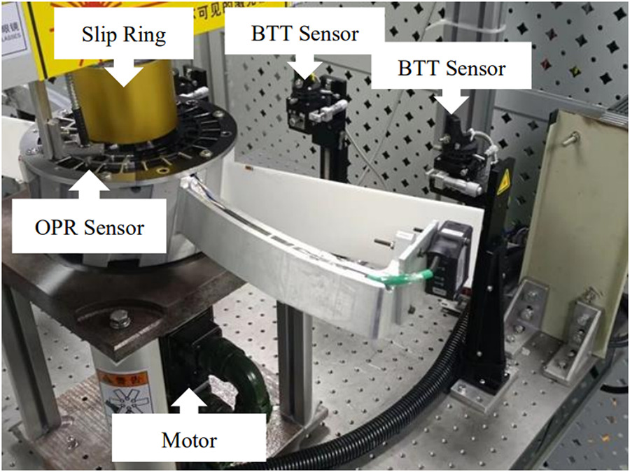
The detailed structure of the experimental platform is shown in Figure 6. The test bench consists of the bench base, a motor, the test wheel, seven circumferential BTT sensors at most, an OPR sensor, the slip ring, the operating platform, and other auxiliary equipment. BTT sensors are circumferentially arranged to measure the blade tip circumferential displacements. During the experiment, the measured blade tip displacement signal was transmitted to a console in real time.
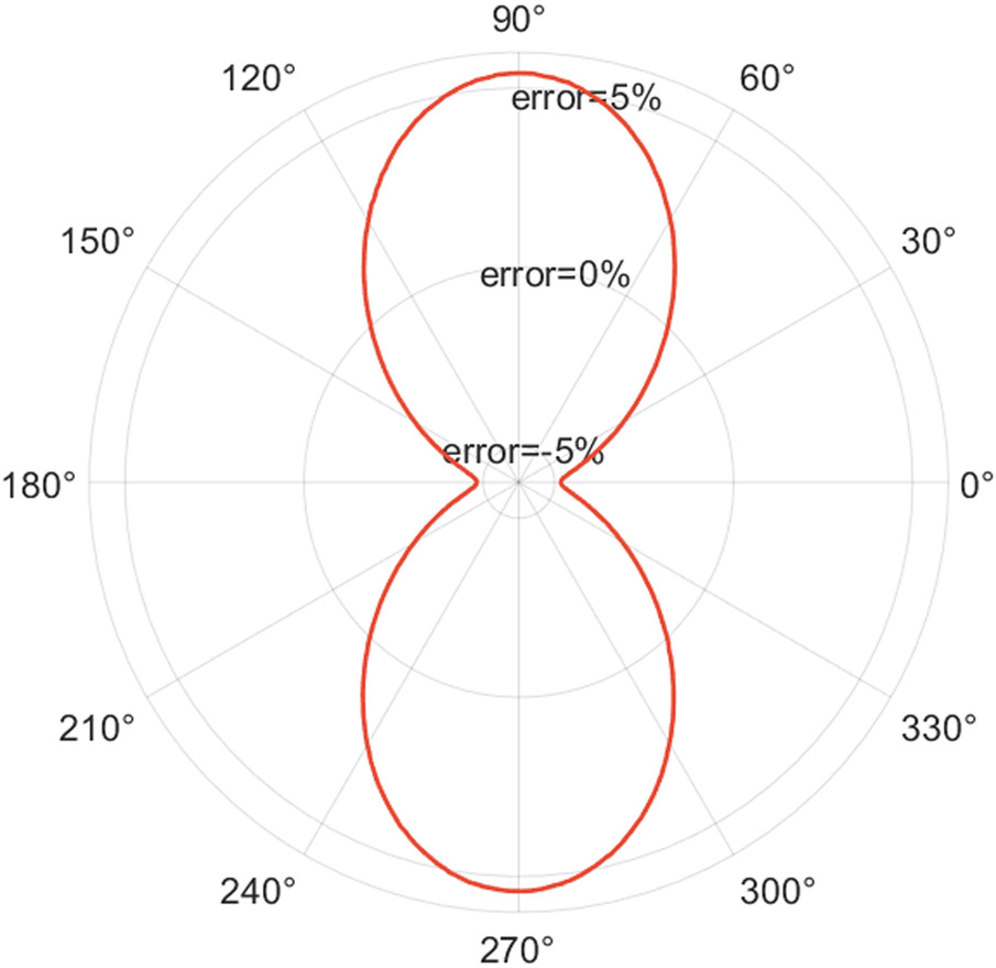
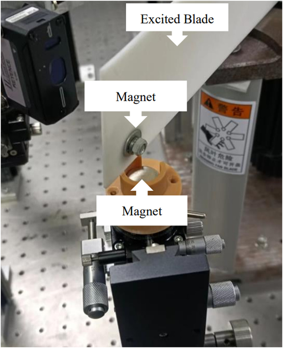
The excitation method of the blade is shown in Figure 7. Permanent magnet was used to excite the blade (Berruti and Maschio, 2012). Two identical magnet stacks were symmetrically arranged around the central axis of the blade disk in the circumferential direction and fastened to the platform by bolts. An identical magnet was fixed at each blade near the tip of blade in order to create the circumferential excitation force with k = 2. The response form of the blade is not changed (Berruti and Maschio, 2012).
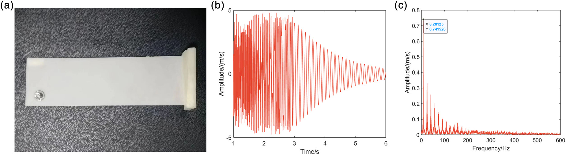
Two straight blades were symmetrically installed on the blade disk. The straight blades were made by 3D printing and the material is resin. The detailed blade is shown in Figure 8(a). The bottom of the blade was fastened by bolts with the blade disk. The blade tip radius r was 320 mm. The direction of blade vibration and the detection direction of BTT sensor are the same. The natural frequency of the blade was measured by a single-point laser vibrometer at stationary state (Ω = 0). The sampling frequency was 1,200 Hz. The blade tip velocity response is shown in Figure 8(b). Fast Fourier Transform (FFT) was used to analyze the velocity response to get the frequency spectrum, as shown in Figure 8(c). The two blades were measured respectively, and it was found that the two blades had good consistency on natural frequency. The first bending natural frequencies of blades were all about 8.28 Hz. Due to the combined effect of stress stiffening and spin softening in the rotation, its natural frequency would be higher than that at stationary state (Kim et al., 2013).
Figure 8.
The straight blade and its natural frequency by Hammering method at stationary state. (a) The straight blade. (b) The velocity response. (c) The frequency spectrum.
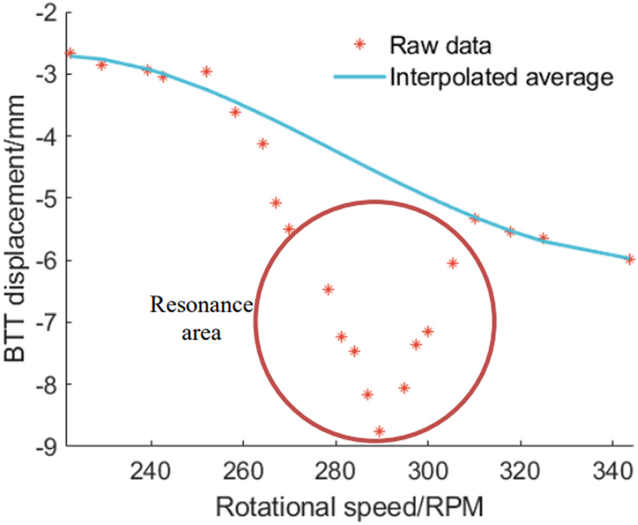
The rotational speed increased from 100 to 700 rpm uniformly and slowly. Part of blade tip displacement data measured by BTT is shown by scatter point in Figure 9. The circumferential installation position of the only BTT sensor used in the casing circumferential coordinate is 168° and the design position of the blade in the rotor circumferential coordinate is −29°. It can be seen that there is obvious characteristic of synchronous vibration near 290 rpm. Due to the material feature of blade and the centrifugal loading of varying rotational speed, the steady offsets of the blade tip are large and cannot be ignored directly. Therefore, we chose the measured blade tip displacement data from the non-resonance area near the resonance area and then spline curve fitting was used to remove steady offset (Mohamed et al., 2019). Because the rotational speed range selected was small, a quartic polynomial was enough to show its characteristics. The interpolation result is shown by the blue solid line in Figure 9. The interpolation result matches well with the measured displacement near the resonance area, and can be used as the mean values of steady offset.
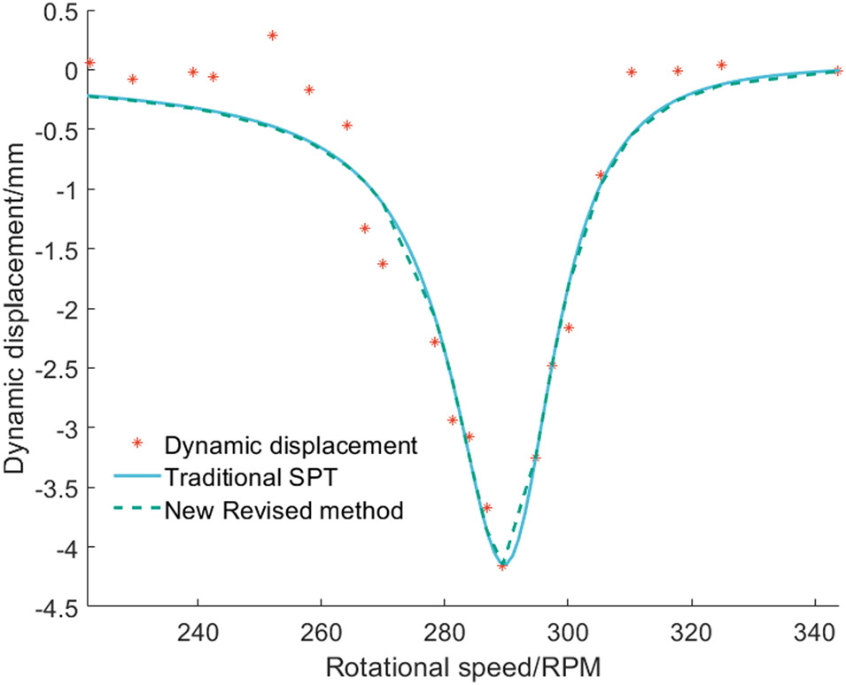
After eliminating the steady offset in the blade tip displacement measured by BTT, the obtained displacement data was used as the dynamic blade tip displacement, as shown by scatter point in Figure 10. Under above conditions, the maximum dynamic blade tip displacement is about 4 mm. The dynamic displacement was used as the left term of traditional SPT [Equation (16)] and the new revised method [Equation (13)]. A nonlinear least square method was used to fit the dynamic displacement and obtain the vibration parameters. The fitted curve is shown respectively by solid line and dotted line in Figure 10. It can be seen that the curves fitted by the two methods have high similarity and are in relatively good agreement with the dynamic displacement data points. Due to the fact that the measured blade tip displacement is relatively small compared to the blade tip radius in the experiment (the maximum value is about 8 mm/320 mm), and k = 2, which is also small and cannot obviously magnify the maximum error. In addition, the installation position of the BTT sensor may correspond to a relatively small error. So traditional SPT could identify the vibration parameters correctly at this time and these two identification results should be relatively similar in theory. Table 3 shows the vibration parameters fitted by these two methods. From the identification results in the table, we can see that the consistency of the vibration parameters identified by these two methods is very high. There is almost no difference, which is basically less than 1%. This is consistent with above theoretical analysis. The experimental results show that the revised method is correct.
Conclusions
Because traditional SPT has some shortcomings in identifying large amplitude vibration, this paper deduces a revised method for both large and small amplitude vibration parameter identification related to BTT actual measurement based on single degree of freedom (SDOF) blade model. The accuracies of two methods for identifying the maximum vibration amplitude are compared by numerical experiment, and the influence of different factors on the error caused by fitting according to traditional SPT for identifying large amplitude vibration is studied. The main source of the error and the error characteristics are also analyzed. Finally, an experimental platform is used to compare the identification results of the revised method and traditional SPT. The main conclusions drawn from the current investigation are shown as follows:
The numerical experiment results show that the accuracy of the revised method for identifying the maximum vibration amplitude is much higher than that of traditional SPT, and the error is basically less than 3%. k (engine order) could also be identified theoretically when k is unknown.
The error of traditional SPT for identifying the maximum vibration amplitude will increase with the increase of the excitation force and the decrease of the damping ratio, and will change periodically in (0.360°) with the change of
A larger Amax or a higher k will magnify the error of identifying the maximum vibration amplitude by traditional SPT. When traditional SPT is used to identify the vibration parameters of large amplitude vibration, the error mainly appears in the damping ratio term.
The experiment results of two methods for identifying low k and small amplitude vibration are compared, and the vibration parameters identified are almost the same, which shows that the revised method is correct.
Nomenclature
y
Dynamic blade tip displacement
ζ
Damping ratio
ω0
Natural angular frequency of blade
F0
Amplitude of excitation force
m
Mass
ω
Angular frequency of excitation force
φ0
Initial phase
ycm
Static shifting of blade tip under the action of force F0
k
Engine order
Ω
Rotational speed (rad/s)
ϕ(t)
Angular displacement of the rotor
tni
Time that the ith blade triggers the only BTT sensor in the nth revolution
Circumferential installation position of the only BTT sensor in the casing circumferential coordinate
Design position of the ith blade without deformation in the rotor circumferential coordinate
tkey,n
Time when the keyphasor sensor is triggered at the beginning of the nth revolution
r
Blade tip radius
xni
Measured blade tip displacement at time tni
Steady offset
Stagger angle of the blade
Amax
Maximum vibration amplitude
Pfitting
The parameter value obtained by fitting according to traditional SPT or the new method
Preal
The given real parameter value in numerical experiment
f0
Natural frequency of blade