
Introduction
Numerical modelling of combustion processes inside combustion chambers play an important role in designing new efficient low emission combustion devices. Especially Computational Fluid Dynamics (CFD) combined with models to predict combustion processes are frequently used during the design of new combustor systems. They are equally important to better understand and improve existing systems.
Reliable applications of CFD-methods require an accurate knowledge of the problem’s boundary conditions. This includes the correct treatment of inlet and outlet boundary conditions as well as the specification of appropriate boundary conditions at the walls of the combustion chamber. For technically relevant flames reliable datasets for the wall temperature distribution at the interior of the combustor do frequently not exist as they are difficult to obtain. Therefore, assumptions have to be made. Usually, adiabatic, isothermal or constant heat flux wall boundary conditions are assumed. Each of these assumptions may, however, result in an inaccurate estimation of the heat loss. An alternative approach is to specify boundary conditions at the exterior of the combustion chamber walls since the exterior is accessed more easily and the environment is less demanding for measurements. Including the exterior boundary in a numerical investigation adds a certain amount of complexity to the simulation as the heat conduction through the solid domain has to be modelled, too. The modelled solid and fluid domains are governed by different differential equations. The sets of equations are coupled mathematically to each other at the interfaces between these domains. Accordingly the coupled set of equations is termed a conjugated problem and therefore the applied method is known as a Conjugate Heat Transfer (CHT) simulation.
In the present work numerical simulations for a model combustor are conducted. The main objective is to solve the CHT problem for this combustor in order to provide accurate wall boundary conditions for the simulation of the fluid domain. To assess the advantages of this approach an additional simulation is performed where constant surface temperatures are used for all walls of the combustion chamber. The model combustor investigated is based on a FLOX® burner and operates at gas turbine relevant conditions. The combustion chamber is optically accessible and well characterized by experiments conducted at the high pressure test rig HBK-S at the Institute of Combustion Technology at the German Aerospace Center (DLR) (Lammel et al., 2017; Severin et al., 2017; Nau et al., 2018; Schäfer et al., 2019; Ax et al., 2020).
As the accurate computation of the combustion chamber inner wall temperature is the main focus of the study, computational results are compared to thermographic phosphor measurements obtained by Nau et al. (2018). By comparing the simulations conducted the influence of the combustion chamber wall temperature on the combustion process is also investigated. Detailed flow field data resulting from Particle Image Velocimetry (PIV) (Severin et al., 2017) and Laser-Raman (Ax et al., 2020) measurements are used to verify the simulation results.
Case description
A schematic overview of the combustion chamber is given in Figure 1 which also shows the placement of the coordinate system. The origin of the coordinate system is located at the centre of the combustor’s base plate. The square cross section of the combustion chamber has a size of 95 × 95 mm2 and a length of 843 mm from the base plate to the circular exhaust gas nozzle. The exhaust gas nozzle is placed concentrically at the end of the combustion chamber. Prior to the combustion chamber lies the mixing duct. The mixing duct is connected to the combustion chamber with a lateral offset of y = −10 mm. Fuel is injected into the preheated air flow of the main burner at the beginning of the mixing duct through a jet in crossflow configuration. The flame can be stabilized by a pilot burner.
Figure 1.
Schematic of the FLOX model combustion chamber with coordinate system and dimensions (mixing-duct and injector geometry are not shown).
Five rows of quartz glass windows (in x-direction) form the confining walls of the square combustion chamber providing optical access for measurements from each side. Each window consists of two plates of stacked quartz glasses which are convectively cooled by an air flow through a gap between these quartz glasses. The windows have a size of 160 × 90 mm2 and are mounted in a copper frame. A more detailed description of the model combustor as well as the high pressure test rig HBK-S is given by Lammel et al. (2017).
Operating conditions
One operating point which is investigated experimentally by Lammel et al. (2017), Severin et al. (2017), Ax et al. (2020) and Nau et al. (2018) is chosen from the experimental data. It represents the case with the most comprehensive data set. The chosen operating point corresponds to case U described in Severin et al. (2017) and Ax et al. (2020). Natural gas with a CH4 content of 92.5–95.8% is used as fuel for this operating point (Lammel et al., 2017). The fuel is injected into the preheated main flow. At this operating point the pilot burner is not used.
Numerical setup
To solve the CHT problem the unstructured finite volume CFD solver THETA (Reichling et al., 2013) of DLR is used. THETA solves the incompressible steady and unsteady balance equations for the fluid in a pressure based manner. For steady-state simulations the SIMPLE algorithm is used. The CHT problem is solved in a partitioned approach. The solver for the solid computes the heat conduction equation in the solid domain whereas the solver for the fluid computes the balance equations of the fluid for the fluid domain. The solvers are coupled at the interfaces of the fluid and solid domain. During the computation the fluid solver passes the calculated heat fluxes to the solid solver. The solid solver then computes the heat equation and returns the calculated surface temperatures to the solver of the fluid. The synchronization events are user definable through specification of the number of iterations for each solver. The simulation continues until steady state in both, fluid and solid is reached.
The computational domain of the fluid includes the combustion chamber, the convergent outlet nozzle as well as the mixing duct and the fuel injector. For the fluid domain the steady-state Reynolds-Averaged Navier-Stokes equations (RANS) are solved using the two-equation k-ω turbulence model (Wilcox, 1988). As the main objective is to compute the combustion chamber’s inner wall temperatures shortcomings of the RANS based approach in predicting the turbulent mixing of a jet in crossflow configurations (Prause et al., 2016) are tolerated. Additionally only half of the domain is considered using the xy-plane as a symmetry plane. A Finite Rate Chemistry (FRC) approach is used to model the combustion processes. Turbulence-Chemistry Interaction (TCI) is taken into account by using an Assumed Probability Density Function method (APDF) to model the thermo-chemical Probability Density Function (PDF) (Gerlinger et al., 2001). Pure methane is used as fuel which approximates the natural gas in the experimental runs. Chemical kinetics is described by the GRI 3.0 mechanism which involves 325 reactions and 53 species (Smith et al., 2020). The overall computational costs are reduced through removal of reactions and species describing the formation of NOx. To gain insight into the OH* distribution and to allow a comparison to measurements, eleven additional reaction steps are added according to Kathrotia et al. (2012). In total 37 species are considered in the simulation. This results in a computational cost of 38 s per iteration for the simulation with CHT and 19 s per iteration for the simulation without CHT (measured on the same computational hardware with identical core counts).
For both simulations the following boundary conditions are applied: The mass flows for fuel and air are available for the chosen operating point and are used in the simulations to specify the velocities at the inlets. The air temperature at the inlet is set to 725 K, the temperature of the fuel is set to 373 K. The walls in the injector geometry as well as the mixing duct and the outlet nozzle are set as isothermal. Furthermore, the combustion chamber base plate temperature is set to a constant value of 600 K. For the simulation without CHT the combustion chamber inner wall temperature is set to 800 K. The boundary conditions applied correspond with former simulations of this case (Lammel and Lückerath, 2017). For the simulation with CHT a solid region containing the combustion chamber is added (see Figure 2). Only the inner quartz glass plate of the windows is included in the computational domain. The gap and the outer quartz glass plates are not modelled. An interface is formed between the fluid domain and the solid domain at the combustion chamber inner walls. The temperature distribution on this interface is computed in the CHT simulation. The thickness of the solid is set to 8.7 mm and matches the thickness of the inner quartz glass plates. The heat transfer coefficient of the convective air cooling between the two rows of stacked quartz glass plates is computed through a Nusselt correlation for pipe flows (VDI, 2006) which is given by
with
and
For the present conditions a heat transfer coefficient of
Table 1.
Properties of quartz glass and copper.
| Parameter | Unit | Quartz glass | Copper | |
|---|---|---|---|---|
| Density | ρ | (kg/m3) | 2,200 | 8,900 |
| Heat conduction | λ | (W/mK) | 1.38–2.68 | 325 |
| Heat capacity | Cp | (J/kgK) | 770–1,050 | 370 |
The fluid domain is meshed as a hybrid grid with structured and unstructured parts. Special care is taken at the combustion chamber inner walls to resolve the thermal and flow boundary layers. A total of 20 prism layers are added to reach a
Results and discussion
Combustion chamber inner wall temperature
The resulting temperature distribution of the CHT simulation is compared to the thermographic phosphor wall temperature measurements conducted by Nau et al. (2018). A total of 17 measurement points for the inner combustion chamber wall are included in the measurement campaign. The measurement points are located on the inner glass plates parallel to the xy-plane. Starting from the burner base plate and continuing in x-direction, 16 measurement points are located at the first window and one measurement point is located at the second window. The positioning of the measurement points as well as the resulting wall temperature distributions from the simulation with CHT are displayed in Figure 3. Figures 4 and 5 show a comparison of the measured inner wall temperatures and the simulation results along four different locations parallel to the x and y axis (see Figure 1 for the location of the coordinate system and the axis orientations). The blue curve represents the simulation results with CHT whereas the circles represent experimental data. A good qualitative agreement between measurement and simulation is found. The temperature in the quartz glass window rises with increasing values of x as the region of maximum heat release is approached. Low temperature areas at the perimeter of the window are caused by the cold copper frame. Therefore, the temperatures in Figure 4 decrease at y = ±45 mm. The drop in temperature which is observed in Figure 5 between x = 160 mm and x = 178 mm is also related to the change of materials (i.e. copper frame and quartz glass window).
Figure 3.
Wall temperature of the combustion chamber resulting from the simulation with CHT. Circles represent available measurement points.
Figure 4.
Comparison between thermographic phosphor measurements (circles) and CHT simulation (line) of the combustion chamber inner wall temperature at constant values of x.

Figure 5.
Comparison between thermographic phosphor measurements (circles) and CHT simulation (line) of the combustion chamber inner wall temperature at constant values of y.
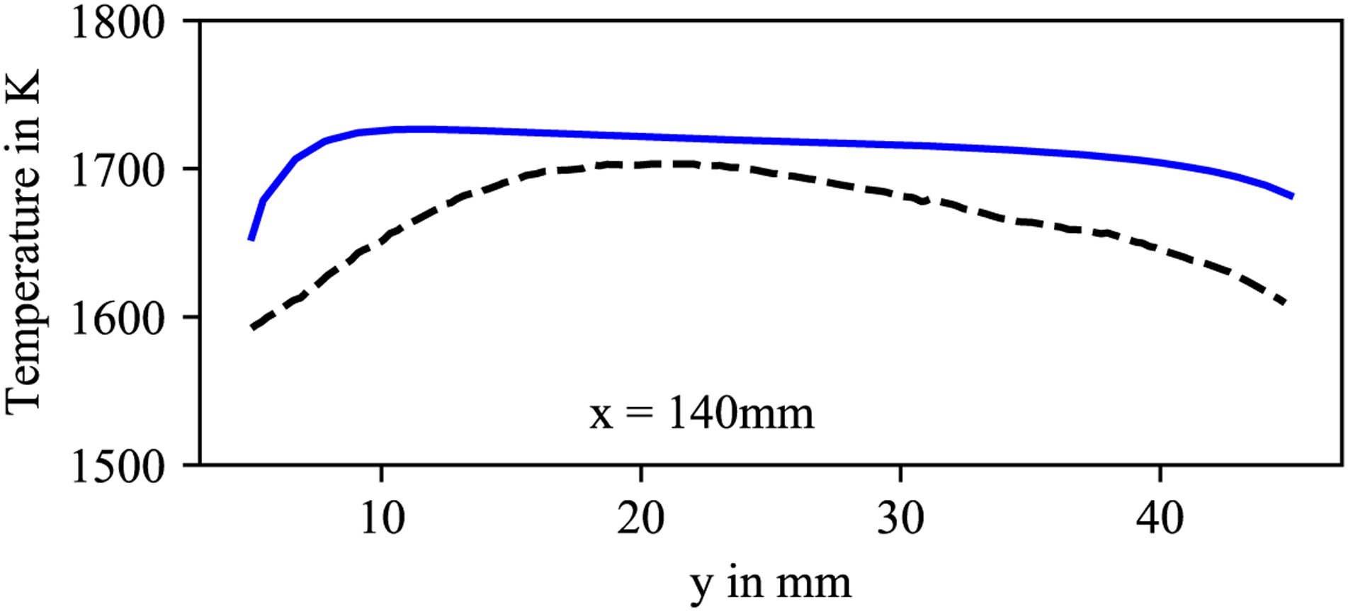
In Figure 4c and d the maximum is slightly shifted towards negative values of y which corresponds to the main injector being located at y = −10 mm. In general the computed temperatures at the wall are slightly higher compared to the measurements which can be attributed to an overall overestimated temperature in the fluid. This is confirmed in Figure 6 where a comparison of measured (black dashed line) and computed (solid blue line) temperatures in the fluid is shown at x = 140 mm (The temperature measurements are provided by Severin et al. (2017)). Additionally, larger deviations in wall temperature are observed for Figure 5a and b than for Figure 5c and d. The discrepancies might again be attributed to the overall overestimated temperatures in the fluid or to the difficulties in reproducing the velocity field with the present RANS based approach which will be discussed in the following section.
Combustion chamber field data
The influence of the combustion chamber wall temperature on the flow field, the flame shape and position is investigated by comparing the simulations with and without CHT to measurement data gained from PIV velocity measurements as well as species data from Laser Raman measurements. The flame position is compared through OH*-Chemiluminescence (CL) measurements. Figure 7 shows a comparison of radial velocity profiles at four different locations along the x-axis. The black dashed line represents the measurement data while the solid red line corresponds to the simulation with CHT and the blue dotted line shows the results of the simulation without CHT. As shown in Figure 7a–c the velocity at the jet core is in good agreement with the measured data. Further downstream the simulations start to differ from the measured results as shown in Figure 7d. There the jet-core velocities are overestimated by the simulations which results in a bigger jet penetration into the combustion chamber compared to the experimental results.
Figure 7.
Comparison between PIV measurement (black dashed line) and simulations with (solid red line) and without (dotted blue line) CHT for constant values of x.
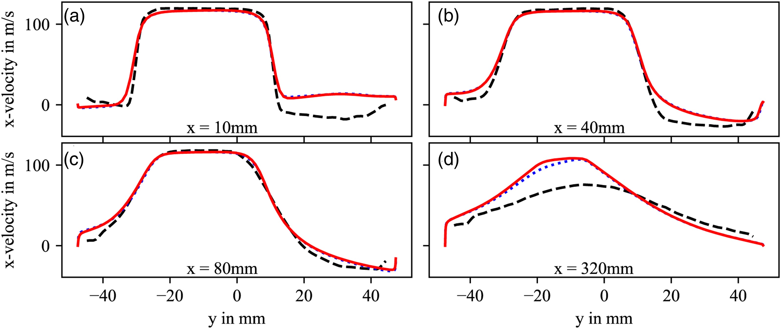
The investigated flame is stabilized by a prominent recirculation zone which is indicated by negative x-velocities. As displayed in Figure 7a and b the recirculation zone is reproduced by the simulation. Compared to the experiment it is located further downstream. Figure 8 shows an axial velocity profile through the recirculation zone at y = 35 mm. Again it is observed, that the start of the recirculation zone in the simulations lies further downstream (here, at x = 25 mm) and appears to be shorter. For all radial velocity profiles shown in Figures 7 and 8 the simulations with and without CHT give an almost identical result which indicates that for the chosen numerical setup, operating point and burner the influence of the combustor wall temperature on the velocity field is insignificant. The present deficiencies in capturing the jet penetration as well as the position of the recirculation zone can, at least partly, be accounted to deficiencies in the applied turbulence model. This can be seen by comparing the data to simulations conducted by Lammel and Lückerath (2017) where more sophisticated LES/RANS (SAS-SST) turbulence models are used.
Figure 8.
Comparison between (PIV measurement (black dashed line) and simulations with (solid red line) and without (dotted blue line) CHT for constant values of y.

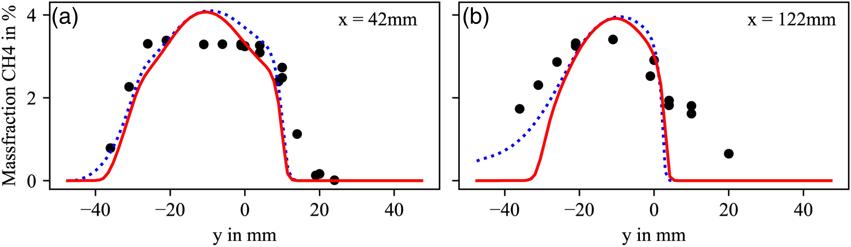
Figure 9 shows radial species profiles for the educt species CH4. Data of Laser Raman measurements as well as the computational results are shown at x = 42 mm and x = 122 mm. The circles indicate the experimental data whereas solid red lines represent the simulation results with CHT and dotted blue curves represent the simulation results without CHT. Major discrepancies in the jet-core region can be observed for the profile in Figure 9a. The measurement suggests a good mixing of fuel and preheated air. In contrast the simulations show a peak in the CH4 distribution which indicates a poorer mixing inside the mixing duct. This is possibly caused by shortcomings of the present RANS approach in capturing the scalar mixing of the jet in crossflow configuration. Further downstream at x = 122 mm in Figure 9b another discrepancy is observed. The simulations show a steep decrease in CH4 concentration whereas the measurement reveals a much smoother decrease. In general, for the experiment it is found that fuel is transported into the recirculation zone. Such an extensive transport is not observed in the simulation.
Figure 9.
Radial species profiles for CH4 at different locations for constant values of x. The circles correspond to the measurement points while the red solid the represents the simulation with CHT and the blue dashed line represents the simulations without CHT.
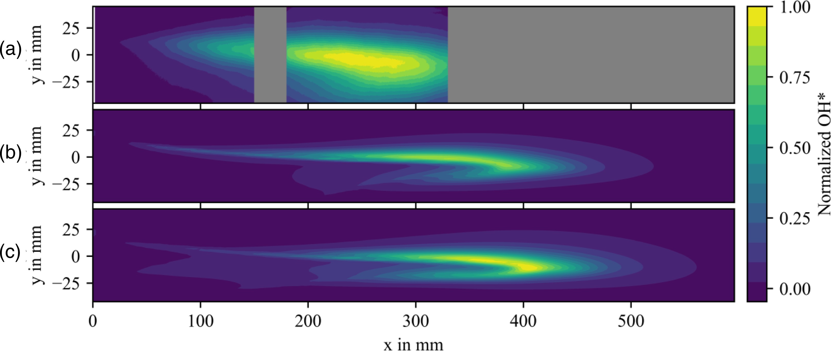
A qualitative comparison between computed and measured flame position is based on a comparison of OH* data. As indicated by Lammel et al. (2017) absolute measurements of OH* concentration are not possible. For a comparison measurement and computations are normalized by their individual maximum value (the same value for the normalization of the simulations with and without CHT is used). In Figure 10 the OH* distribution is displayed for (a) OH*-CL measurements, (b) simulation without CHT and (c) simulation with CHT. It is clear that in comparison to the experiment, the simulation results show a much thinner flame which extends further into the combustion chamber. Additionally, the area of maximum OH* concentration is smoother and broader in the experiment compared to the simulation. This is consistent with observations made in Figures 7 and 9 concerning the velocity and CH4 distribution. For the simulations the fuel jet penetrates deeper into the combustion chamber. Consequently, mixing appears to be poorer which results in a more discrete flame compared to the experiment.
Figure 10.
Comparison between OH*-CL measurement (a) and simulations without (b) and with (c) CHT. Absolute values for each contour plot are normalized by the individual maximum value. Greyed regions represent areas with no data available.
Comparing Figure 10b and c only minor differences are found between both simulations. The flame position is almost identical. Compared to the simulation without CHT a slightly higher OH* concentration is found for the simulation with CHT. This can be related to higher temperatures in the heat release zones for the simulation with CHT. Moreover, for negative values of y heat release still occurs further upstream where higher wall temperatures are found. In this area further differences between both simulations are found. Figure 11 shows a comparison for the OH-radical for both simulations in the region of y < 0 mm and x < 400 mm. Figure 11a displays the resulting distribution for the simulation without CHT whereas Figure 11b shows the results of the simulation with CHT.
Figure 11.
Comparison for the OH-radical distribution for (a) simulation without and (b) simulation with CHT. The data is shown for y < 0 mm and x < 400 mm.
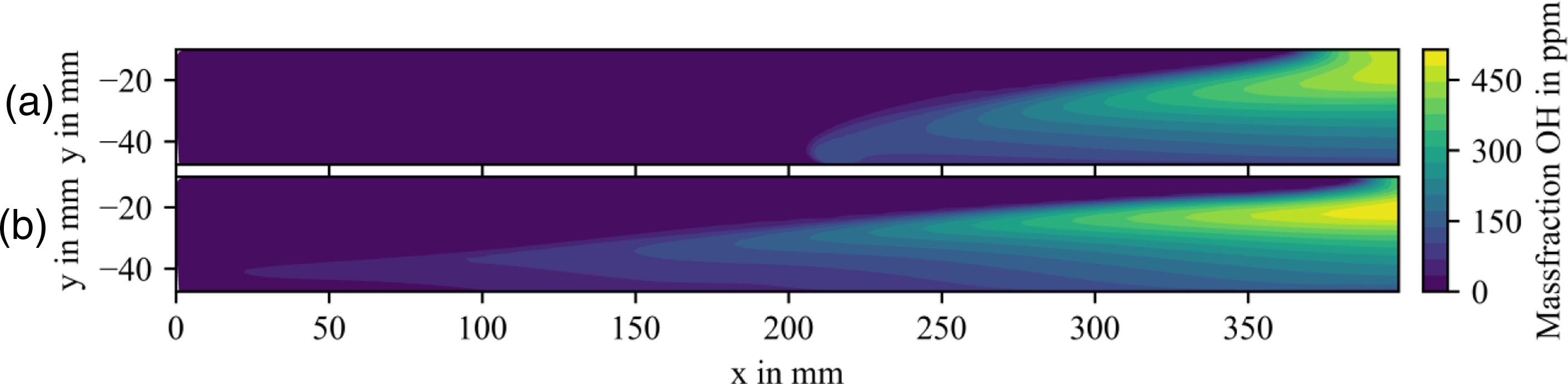
The higher wall temperatures in the simulation with CHT favour OH formation further upstream. The same observation is made for other radicals which are not shown here. The differences in wall heat transfer also influence the formation of pollutants. Table 2 shows an evaluation of CO at the exit of the combustion chamber and compares computational results to the measured CO emission of Severin et al. (2017). The simulation without CHT underestimates the measured CO emission by a factor of two, whereas the simulation with CHT captures the experimental data accurately. For the present burner the accurate computation of the wall temperature distribution is therefore of major importance for computing CO emissions correctly.
Table 2.
Comparison of CO emissions at the exit of the combustion chamber.
| Case | without CHT | with CHT | Measurement | |
|---|---|---|---|---|
| CO nomralized to 15% O2 | (ppm) | 2.11 | 4.29 | 4.2 |
[i] See Severin et al. (2017) for measurement data.
Conclusions
A single injector FLOX® type model burner is simulated and compared to measurement data. The simulations include the heat conduction through the combustor’s confining walls. Computed surface temperatures show an overall good agreement with measured temperature data. Therefore, the presented method offers the ability to impose accurate boundary conditions at the combustor inner wall which otherwise would need to be approximated due to a lack of information. In some points larger discrepancies in computed wall temperature compared to measurement data are found than for others. To clarify the origin of these discrepancies more detailed experimental data on temperature and velocity distribution in the gas phase as well as further numerical simulations are required.
The comparison of the computed velocity field, species distributions and flame position to experimental data shows some deficiencies in the present RANS based approach. The qualitative aspects like flame lift-off and flow recirculation are, however, captured by this model.
Comparing the simulations with and without CHT, the flame position for this case does not seem to be affected by the treatment of the wall boundary conditions. Additionally, the influence on the velocity field seems to be insignificant. However, differences are observed in the field of composition. Especially the influence on emissions such as CO is significant and better results are obtained by the use of CHT.
To improve the prediction of flame position as well as scalar mixing more sophisticated approaches like large-eddy simulations (LES) are necessary (Lammel and Lückerath, 2017). As the available experimental wall temperature dataset is limited to a single quartz glass window, the computed wall temperature distribution could be used as a boundary condition for further simulations. Alternatively the applied method could be used directly in conjunction with an LES simulation.