Numerical framework

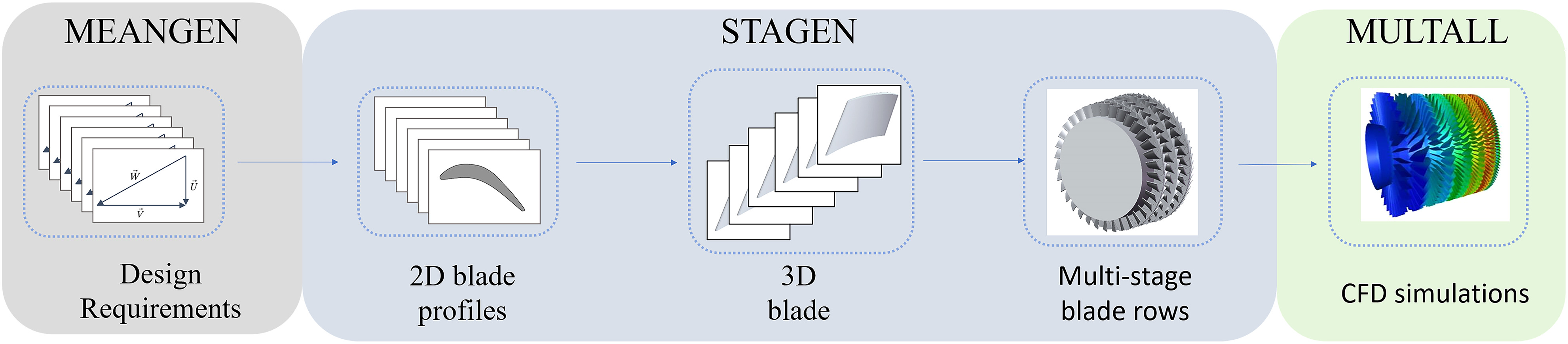
All the CFD results reported in this paper were obtained using the Multall turbomachinery design system in-house flow solver. The system comprises of three related programs developed using FORTRAN77: MEAGEN, STAGEN, and a 3D solver. MEAGEN performs a 1D calculation to obtain velocity triangles, set annulus boundaries, generate initial blade shapes, and twist them for a free/forced vortex design. The output file from MEAGEN serves as an input file for STAGEN, which defines the blade shapes. The 3D blade is generated by stacking and combining 2D blade shapes into stages. Finally, the Multall system reads the input file written by STAGEN and performs a 3D multistage calculation to predict the detailed flow pattern and overall performance. The roadmap of the design system is shown in Figure 1.

Figure 1.

Roadmap of turbomachine aerodynamic design process using Multall.

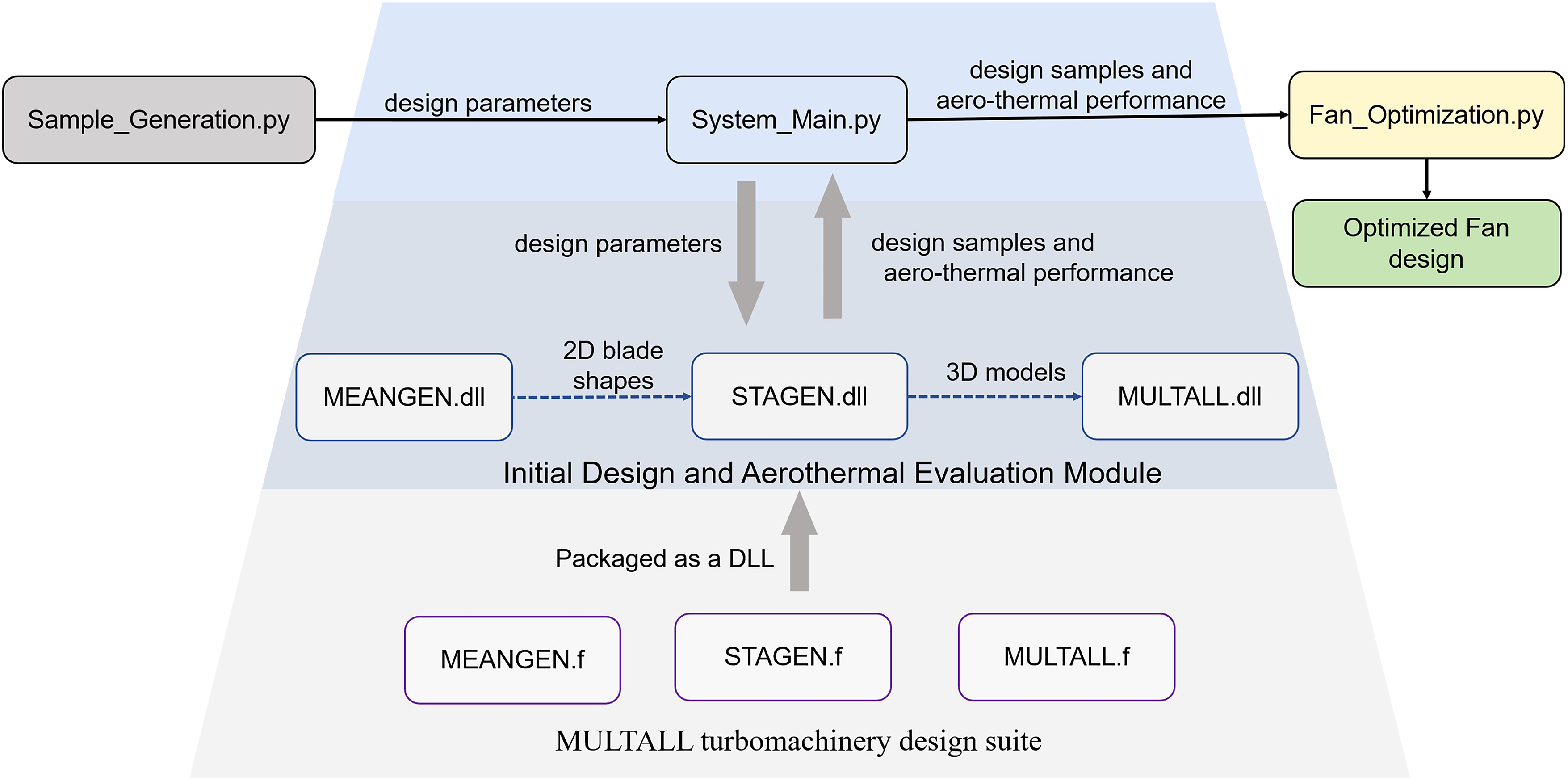
To automate the process, it would be beneficial to integrate the Multall turbomachinery design system within a Python-based blade optimization framework. One way to achieve this is by using function libraries, which are simple and cost-effective. Using a dynamic link library (DLL) instead of a static link library allows for repeated calls without wasting resources and can be changed without recompiling. Given the system’s structure, it is necessary to convert the three linked programs into DLLs, each corresponding to a specific aspect of the system. The main program can then call these DLLs in sequence, as shown in Figure 2. This approach enables more seamless integration of the Multall design suite with the Python-based optimization framework, making it easier for users to design and optimize turbomachinery blades.

Figure 2.

The Python-based blade optimization framework with integration of Multall.

Target design space and sampling strategy

This section describes the exercise conducted on a single-stage ducted fan. It focuses on generating multiple blade-shape design samples using Gaussian random sampling. First, a design space of 16 parameters is established, listed in Table 1. The blade-shape design parameters serve as input parameters, while the three aero-thermal performance metrics are objectives to train the active subspace. This approach helps identify the most critical input parameters that impact the performance metrics most, allowing for more efficient optimization of blade designs.

The design parameters are defined around normal values and sampled using Gaussian random sampling with N = 344. The range of each parameter is listed in Table 1. Each sample set x^j is a vector of 16 dimensions and the value of each element falls within the range [xl,xu], its description is:

x^j represents the vector of jth samples of input parameters. μ is a m-vector and equal to the average of xl and xu, shown in Equation (3). According to sigma rules, σ is defined:

As to the sample size requirement, the size of samples must be larger or equal to G=αk(m+1)In(m). An oversampling factor, α, between 2 and 10 is typically selected in practical applications. This ensures that the sample is large enough to capture the variability in the data and provide statistically significant results. Lastly, a normalization process is employed to ensure that the analysis is not affected disproportionately by parameters with larger values. The normalization process involves transforming the input parameter vector x^j of each sample to a standard range. This standard range centers all the transformed parameters at zero, making them dimensionless and giving them equal weight in the analysis. The standard range of the transformed parameters is [−1,1]m, where m is dimension of the design space. The normalization is carried out using Equation (4).

Active subspace identificaiton

This study carried out active subspaces for three critical aero-thermal parameters of the ducted fan. The first objective is to optimize the adiabatic efficiency of the single-stage fan, which is the primary focus of the study. The second objective is the flow capacity of the fan, which is restricted in this study. The third objective is to ensure that the pressure ratio of the fan is equal to the pressure ratio of the baseline design.

In term of adiabatic efficiency

An active subspace for adiabatic efficiency is sought to capture its variation in 16-dimensional space with fewer dimensions. The goal is to construct an active subspace that reduces the dimensionality to the expected dimension, which is determined by evaluating the gap in the eigenvalues (Constantine, 2015).

The first step is to calculate the subspace eigenvalues of each dimension using gradient decomposition. If gradients are not available, finite difference approximations can be used to obtain approximate values of the gradient. In this study, the small design space makes it feasible to use finite difference approximations. eigenvalues λk and corresponding eigenvectors ηk are obtained for each dimension k = 1, ……, 16. The eigenvalues are then plotted on a log scale, as shown in Figure 3. Figure 3(a) shows that the largest gap lies between the 1st and 2nd index, indicating that the most suitable active subspace is one in this case. Figure 3(b) plots the estimated eigenvalues along with the bootstrap intervals and shows that the calculation error in the scenario of a single dimension is the smallest.

Figure 3.

The eigenvalues (a) and subspace errors (b) of adiabatic efficiency active subspace.

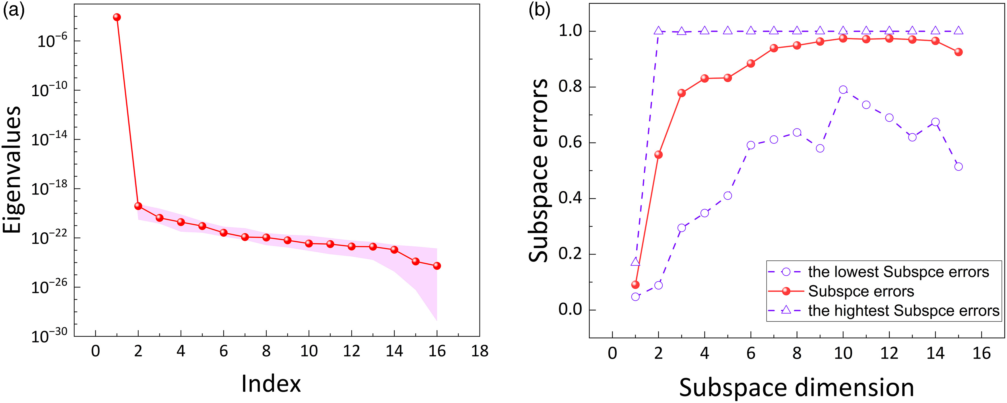
The main idea behind subspace dimensionality reduction is to use matrix multiplication between the input parameter vector and a tall transformed matrix, reducing the high dimensionality of m to a lower dimensional s. The transform zj=MTxj is called a forward map, where zj∈Rs, xj∈Rm, M∈Rm×s. It maps the m-dimensional design vector to an s-dimension coordinate. The transform matrix is determined by the eigenvalues and eigenvectors, and a large gap between the sth and (s + 1)th eigenvalue indicates a strong univariate trend between the objective yi and the combined matrix of the first s eigenvectors, M=(η1,η2,⋯,ηs)Txj (Constantine, 2015). In this study, the first eigenvalue was found to have the largest gap, indicating that the transform matrix M1 for the efficiency active subspace is a matrix stacked with the first eigenvector. This matrix is described:

(5)

M1=(0.431,−0.091,0.188,0.783,−0.071,−0.007,−0.013,−0.001,−0.288,−0.075,−0.164,−0.146,−0.111,0.199,0.484,−0.001)T

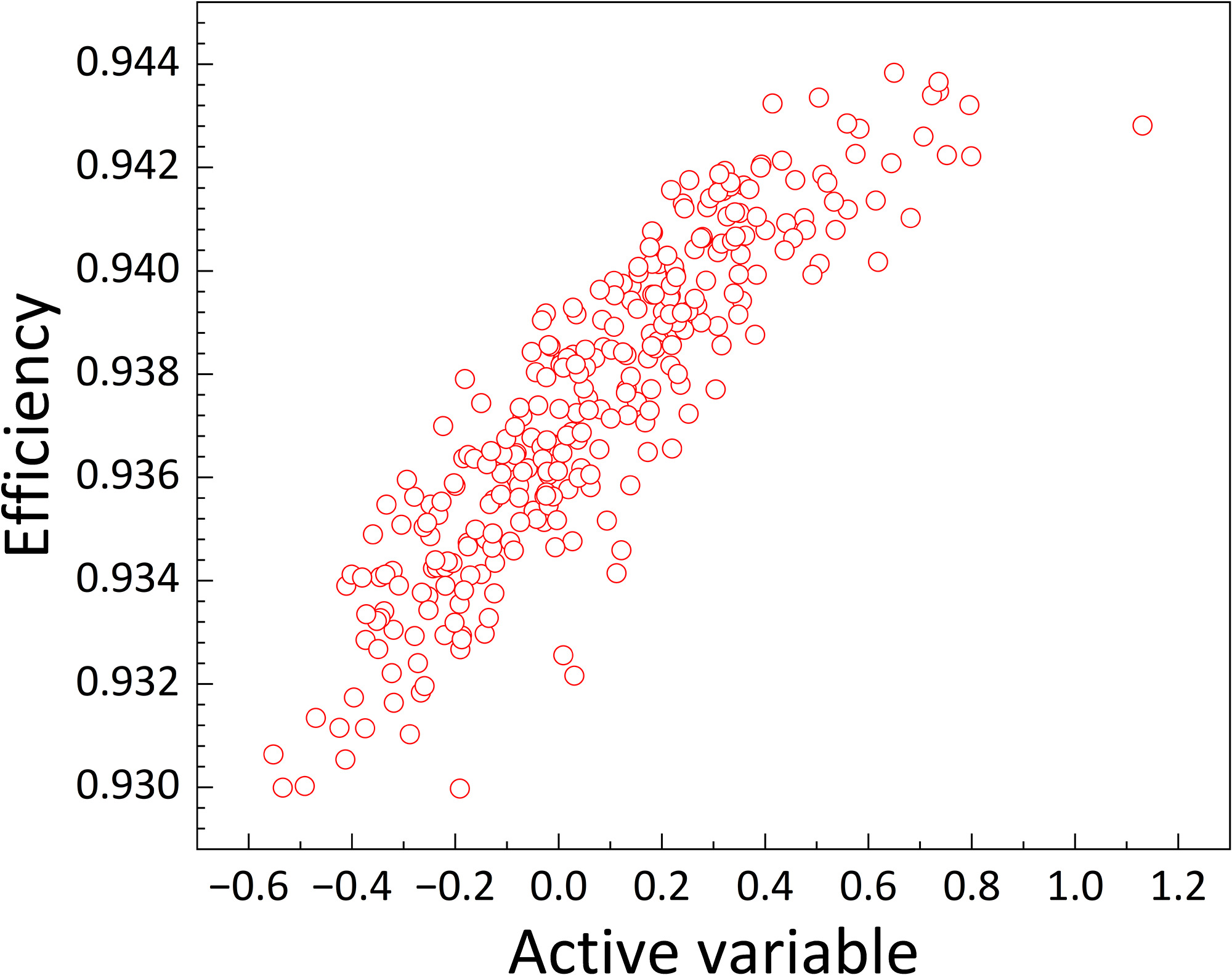
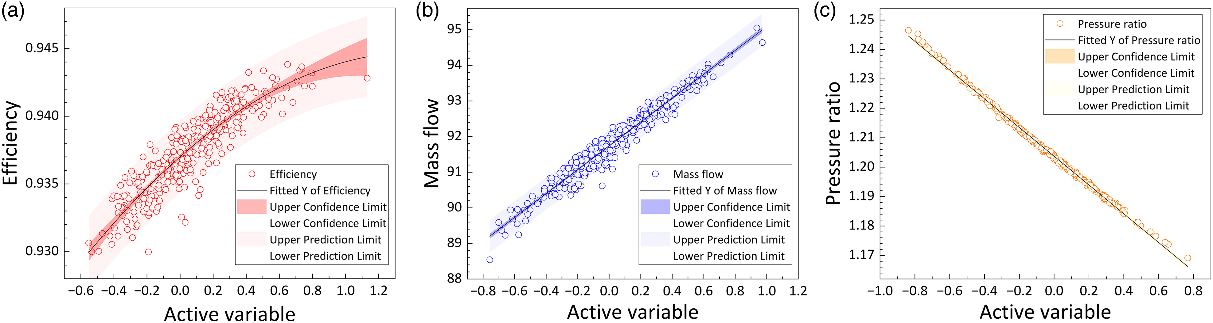
Furthermore, Figure 4 shows the relationship between the forward map z and the adiabatic efficiency y1. The figure depicts a manifold relationship between the map of 16 design parameters and adiabatic efficiency y1, indicating that the most significant direction of the design parameters space, along which the largest change of the adiabatic efficiency occurs, has been successfully identified. As shown in the figure, adiabatic efficiency varies as a quadratic function curve along a single vector in the 16-dimensional design space. This confirms that the active subspace has reduced the high-dimensional design space to a lower dimensional space capturing the most significant variations in the objective.

Figure 4.

Scatters of adiabatic efficiency in efficiency active subspace.

In term of mass flow rate

Following the same procedure, the active subspace for mass flow is identified. Same as the adiabatic efficiency, the largest gap between adjacent eigenvalues in the scenario of mass flow also lies between the 1st and 2nd index, shown in Figure 5(a). Additionally, a single dimension also yields the smallest error, shown in Figure 5(b). Lastly, the transform matrix, M2, is obtained. The scatter plot, Figure 5(c), indicates a fairly linear connection between the subspace M2Tx and mass flow y2.

Figure 5.

The eigenvalues (a), subspace errors (b) and scatters of mass flow (c) in mass flow active subspace.

(6)

M2=(0.036,0.272,−0.165,0.293,−0.018,−0.008,0.017,0.08,0.845,0.102,−0.253,−0.126,−0.109,−0.059,−0.003,−0.047)T

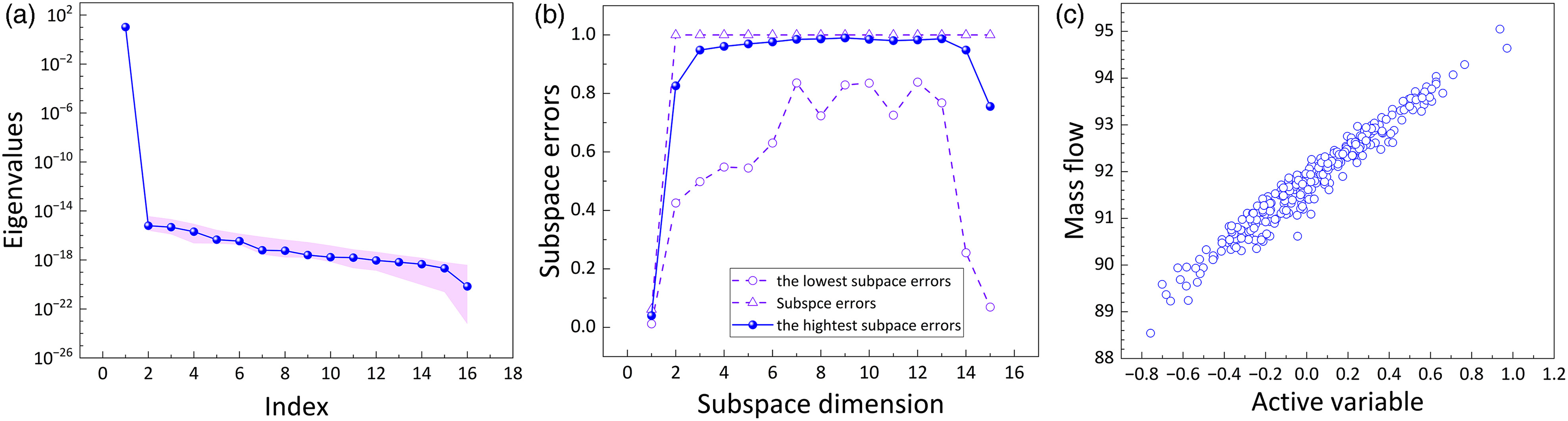
In term of pressure ratio

Lastly, the active subspace for the total-to-total pressure ratio is identified. Similarly, the largest gap between adjacent eigenvalues in the scenario of total-to-total pressure ratio also lies between the 1st and 2nd index, shown in Figure 6(a), and a single dimension yields the smallest error, shown in Figure 6(b). Lastly, a linear connection between the subspace M3Tx and mass flow y3 was spotted, shown in Figure 6(c).

Figure 6.

The eigenvalues (a), subspce errors (b) and scatters of pressure ratio (c) in pressure ratio active subspace.

(7)

M3=(2.55e−2,−6.22e−4,−4.41e−1,−8.84e−1,8.57e−4,−1.01e−3,1.57e−3,−3.92e−4,−1.47e−1,1.05e−2,4.29e−2,8.02e−3,4.29e−3,1.44e−2,−9.69e−4,7.41e−3)T

To summarize, this section discusses the use of active subspaces to identify dominant directions in a high-dimensional design space. By using this technique, the authors were able to reduce the dimensionality of the design space and identify the most significant design parameters affecting the performance of a ducted fan. Results show that active subspace exists for fan adiabatic efficiency, mass flow rate, and total-to-total pressure, and the most suitable dimension for all three parameters is one. For adiabatic efficiency, a manifold relationship between the subspace and adiabatic efficiency is observed, where the adiabatic efficiency varies as a quadratic function curve along a single vector in the 16-dimensional design space. A fairly linear connection between the subspace and the parameter is concluded for mass flow and total-to-total pressure ratio.

Fidelity analysis

Despite the promising result presented in the above section, questions remain such as independence of the active subspaces, sensitivity of parameters, and accuracy of manifold modelling. This section investigates the fidelity of the active subspace approach. First, to verify the independence of the previously identified active subspaces, additional data samples can be generated randomly in the design space and used to compute the subspaces again. If the resulting subspaces are similar to those computed earlier using the limited number of samples, it can be concluded that the subspaces are independent of the specific data samples used and represent the dominant direction of the objective in the whole design space. To investigate the sensitivity of various design parameters, the gradient of the objective function for each design parameter can be calculated using the active subspace. This will provide insight into which design parameters impact the objective most and can be used to guide the optimization process. Lastly, a manifold model can be fitted to the data in the active subspace, which can be done using linear regression for a linear model or polynomial regression for a quadratic model. The accuracy and fitness of the model can be evaluated using statistical metrics such as the R-squared value and mean squared error.

Independence of active subspace

Two questions need to be addressed to verify the independence of the active subspaces from the data samples. The first question is whether the active subspaces would differ with different sample contents for the same sample size, and the second question is whether the sample size can affect the result of the active subspaces. This section uses a series of samples of different sample counts to investigate the effect of the sample size on the active subspaces. The recommended sample size G=αk(m+1)In(m) is used to set the upper and lower bounds for the smallest sample size for finding a functional subspace. The constant α is an oversampling factor typically chosen to be between 2 and 10. Gaussian random sampling is used to select numerous data samples from the design space, with sample sizes ranging from 100 to 500 with an interval of 50. These samples are used to perform simulations and obtain the objective metrics for finding the active subspaces. The results for the adiabatic efficiency subspace are shown in Figure 7. There is little difference in the eigenvalues for sample size varying from 100 to 500, shown in Figure 7(a). The subspace error and eigenvector components also change within the permissible error range, as shown in Figures 7(b) and 7(c).

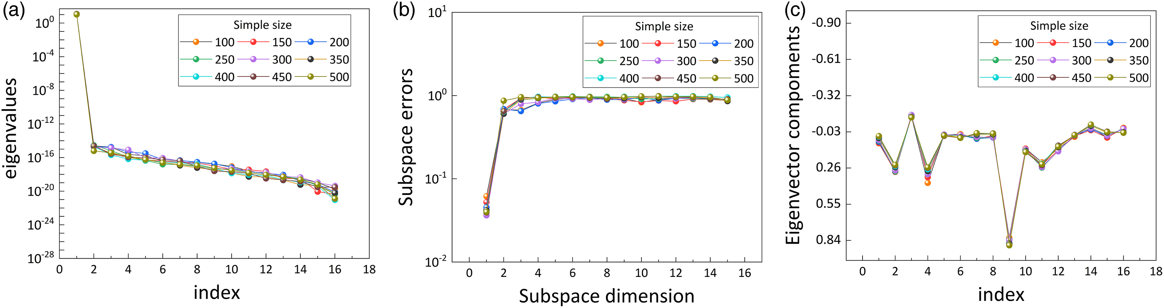
Figure 7.

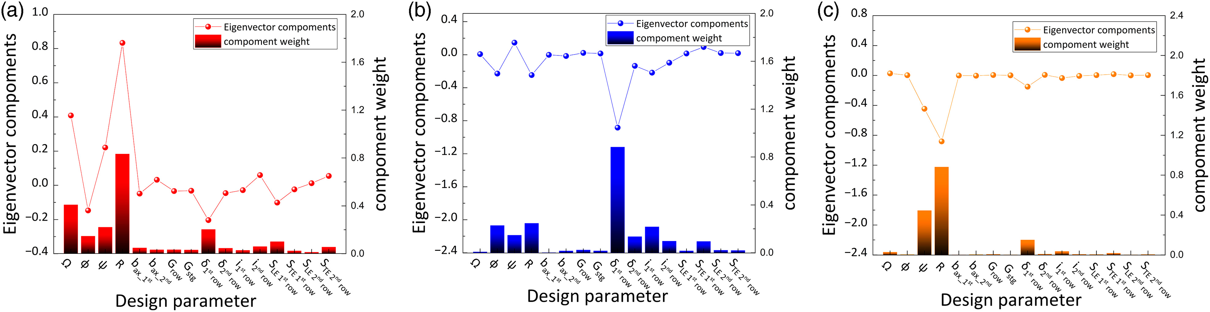
The independence verification for adiabatic efficiency subspace: eigenvalues (a), subspace errors (b) and eigenvector components (c).

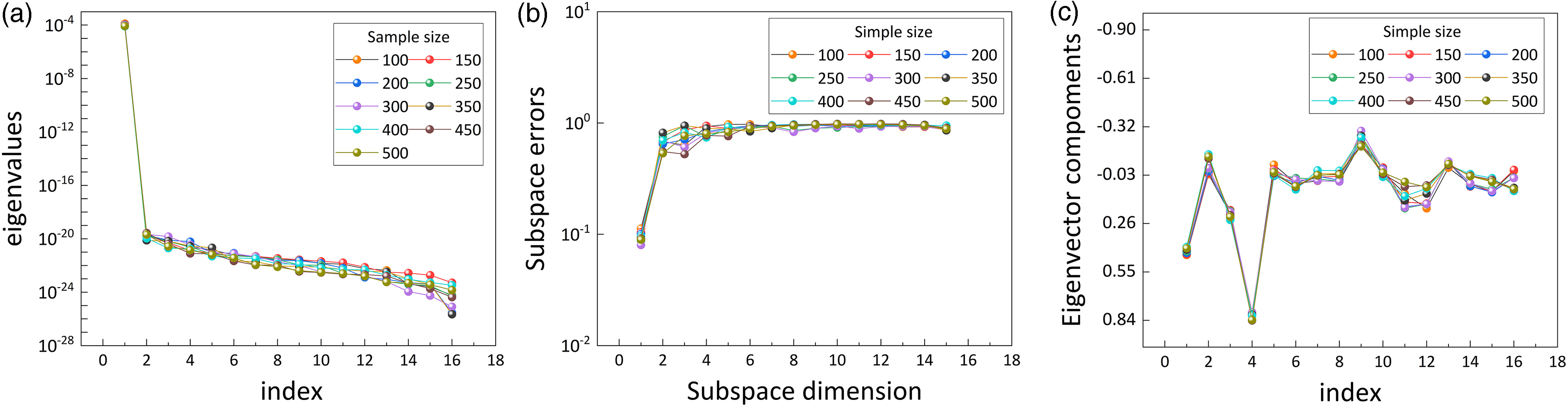
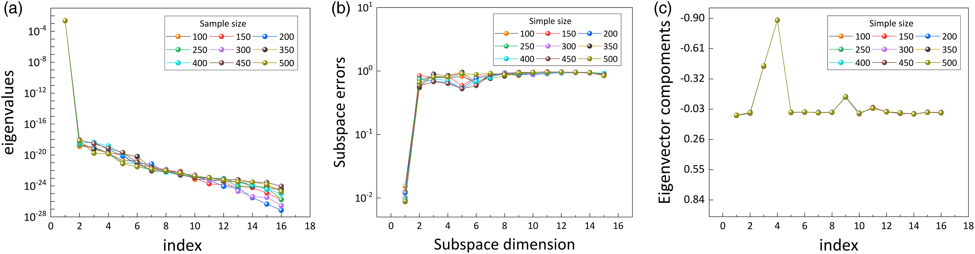
Additionally, the independence of the mass flow rate subspace is also shown in Figure 8. Figures 8(a) and 8(b) demonstrate no significant difference in the existing eigenvalues and subspace errors for each dimension among different sample sizes. The subspace components also fluctuate only slightly within a very small range. Lastly, Figure 9 shows that the pressure ratio subspace is almost unaffected by the training samples, as the curve remains the same as the sample size increases. These results demonstrate that the active subspaces discussed in Section 2.3 are independent of the data samples used in the calculation process.

Figure 8.

The independence verification for mass flow subspace: eigenvalues (a), subspace errors (b) and eigenvector components (c).

Figure 9.

The independence verification for pressure ratio subspace: eigenvalues (a), subspace errors (b) and eigenvector components (c).

Sensitivity analysis in terms of parameters

In Section 2.4.1, it is demonstrated that the elements of transformed matrices M are independent of the size and content of the samples used in the calculation process. These matrices are used to transfer the 16D design space to a 1D space, with aero-thermal performances serving as the objective metric. This means that the active subspaces are also a combination of all design parameters, with coefficients linking each parameter to the significance of the objective. A larger coefficient indicates that the objective value is more sensitive to changes in the related parameter. Figure 10 plots the eigenvector components of each active subspace and the component weights of all design parameters. In Figure 10(a), the adiabatic efficiency active subspace has 16 components associated with the 16 design parameters. The height of each column in each index corresponds to the influence of the parameters on adiabatic efficiency. The largest perturbation is caused by Radius, followed by Reaction, First-row deviation angle, and so on. Figure 10(b) shows the distribution of elements for vector M2, which represents the contribution to the dominant direction. This figure shows that design variables such as First-row deviation angle, Radius, and Flow Coefficient have greater weights in the direction. In contrast, Second-row LE QO angle, Blade Axial Chord 2nd row, and Stage Gap have less influence. Lastly, Figure 10(c) indicates the significance of the components corresponding to M3 in the active subspace. Increasing the pressure ratio is mainly achieved through changes in the Radius and Loading Coefficient, with the remaining design variables contributing less to this objective. Overall, these findings highlight the important role that each design parameter plays in determining the overall performance of the ducted fan, as well as the usefulness of the active subspace methodology in identifying the most critical parameters.

Figure 10.

The eigenvector components and corresponding weight of desigen paramenters: effciency active subspace (a), mass flow active subspace (b), pressure ratio subspace (c).

Fitting curve of active subspace

This section uses polynomial fitting to build fitting curves in the active subspaces. Polynomial fitting aims to establish a functional relationship between the map z=MTx and the objective y using a polynomial with degree n.

(8)

y=a0+a1z+a2z2+⋯+anzn

where n can be any positive integer.

The scatter plots in Figures 4(a), 5(c), and 6(c) show the distribution of design samples in each active subspace. Based on these scatter plots, linear or quadratic responses may fit the trend of the scatter distribution very well. Therefore, using first-order polynomial and secondary-order polynomial to fit the objectives y1,y2,y3 in their subspaces.

(9)

y=a0+a1z

(10)

y=a0+a1z+a2z2

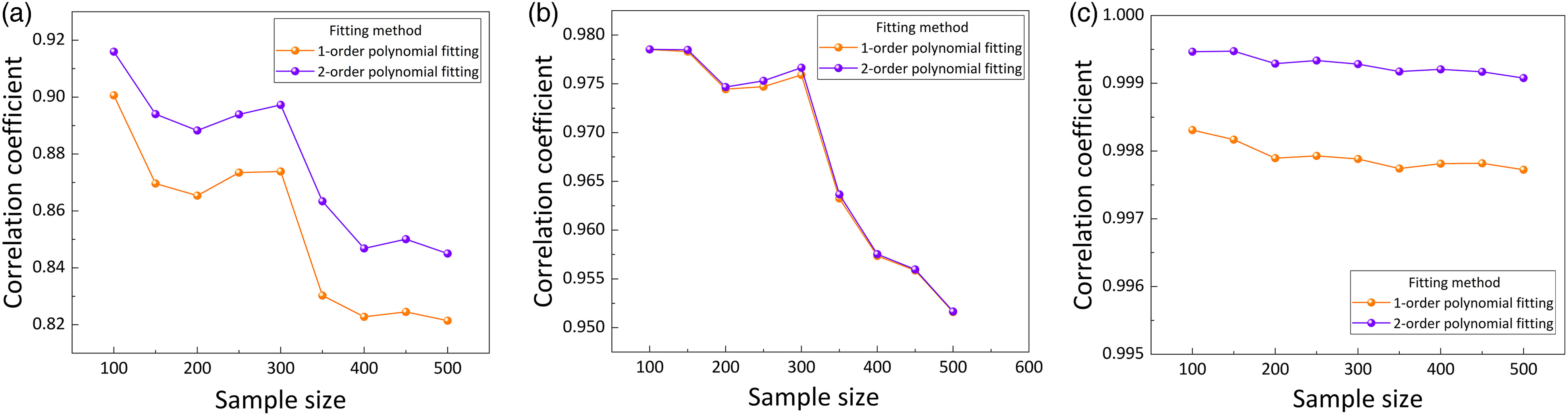
To compute the coefficients associated with the models, Equations (9) and (10) are built using samples. To choose the best function curve fitting the plots, the correlation coefficients of the two functions in all active subspaces must be compared. Figure 11(a) compares the correlation coefficients of the first-order and second-order polynomials with different sample sizes in the efficiency subspace. The graph shows that the line of the second-order polynomial fitting is above that of the first-order polynomial from beginning to end, indicating that the quadratic curve has a stronger correction of sample scatters in the efficiency subspace. Furthermore, the quadratic curve tends to be stable, and the coefficients in the line still drop as the sample size increases. Thus, the second-order polynomial fitting is chosen, and the related coefficients are computed using Equation (11).

Figure 11.

Correlation coefficients of two fitting curves in different sample size: adiabatic efficiency (a), mass flow (b) and pressure ratio (c).

(11)

f1=0.937+0.0104z1−0.00433z12

where f1 is the proper function of efficiency active subspace based on 300 training samples. The coefficient R12 is 0.873. The polygonal lines in Figures 11(b) and 11(c) show a small distance, and fitting curves of different sample sizes all share high coefficients. Considering calculation convenience and the light influence of the two constraint objectives to optimize blade efficiency, mass flow and pressure ratio active subspaces use first-order polynomial fitting, shown in Equations (12) and (13).

(12)

f2=91.739+3.333z2

(13)

f3=1.204−0.0491z3

where f2 and f3 are the appropriate functions of mass flow and pressure ratio active subspaces, respectively, both calculated using 300 samples. Their coefficient R22 and R32 are 0.972 and 0.998, separately. Finally, the fitting curves with sample scatters are displayed in Figure 12.

Figure 12.

Fitting curves in active subspace: adiabatic efficiency (a), mass flow (b) and pressure ratio (c).

Optimization of a single-stage fan blade

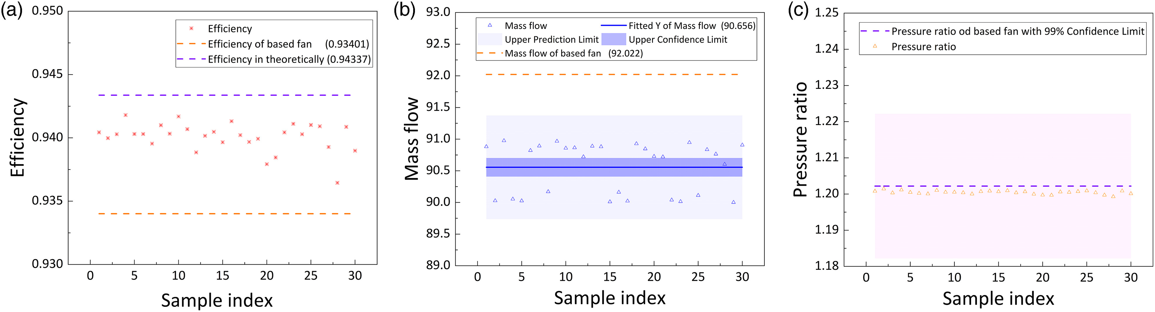
This section focuses on optimizing a single-stage fan blade with specific parameters shown in Table 1. Using the Multall solver, the adiabatic efficiency, mass flow, and pressure ratio of the fan are computed as 93.401%, 92.022 kg/s, and 1.202, respectively. The main objective of the optimization is to maximize the adiabatic efficiency while keeping the mass flow and pressure ratio constant. An equation group that includes constraint equations from the mass flow and pressure ratio active spaces and an objective equation from the efficiency space is constructed to achieve this objective. The equation assembly is presented in Equation (14).

Prio to solving the above equation assembly, it is important to analyze the monotonicity of the objective function with respect to the constraints. By examining the plot of the quadratic function, it is evident that the objective function first increases and then decreases at the axis of symmetry −b/2a=1.205. Therebefore, it is necessary to get the value range of z1, the other maximizing problem shown in Equation (15).

This optimization problem is solved using the simplex algorithm, and the resulting design vector x′max is shown in Equation (16), which corresponds to the maximum value of z1. As the maximum value of z1 is 1.567, which is greater than the axis of symmetry at 1.205, it can be concluded that the maximum efficiency of 94.337% is achieved when z₁ = 1.205.

Furthermore, Equation (14) can be transformed as a group of indefinite equations, shown in Equation (17).

Since three equations can only solve for three unknowns, the three most sensitive parameters – radius, first-row deviation angle, and loading coefficient – are selected as unknowns in Equation (17). The other parameters are considered as known values obtained by average random sampling in the design space. However, it was found that Equation (17) was difficult to solve by directly sampling the entire design space. Only a small region in the design space could be mapped to 1.20471 or greater in the efficiency active subspace. Therefore, an effective method was to limit the sample space to the vicinity of x′max. Each design parameter was selected from a region centered on x′max in the design space. The length of the region in each dimension was set to be 10% of the length of the design space.

Lastly, a total of thirty sets of unknowns were sampled using average random sampling, and by solving Equation (17), 30 optimized fan designs were produced. The aero-thermal performances of these designs were then calculated using the Multall solver, and the results are shown in Figure 13. Figure 13(a) shows that the adiabatic efficiency of the optimized fans was, on average, higher than that of the baseline design, but it did not reach the highest theoretical efficiency. Some issues with the fitting curves may need to be addressed to improve efficiency further. Figure 13(b) indicates that the mass flow of the optimized fans was slightly different from the base mass flow, but it centered around 90.656. Based on this result, the authors proposed changing the aimed mass flow from 92.022 to 93.388, as mass flow has a strong linear changing tendency. On the other hand, the pressure ratios of the optimized fans remained largely unchanged compared to those of the base fan, as shown in Figure 13(c). To correct the target value of the indefinite equation, the authors first noticed that the scatter distribution on the horizontal axis in Figure 11(a) was limited below 0.8, which made the fitting curve heavily dependent on the data below 0.8 and imprecise at the largest value point. To address this issue, the authors set groups of random aimed values above 0.8 of M1x in Equation (17) and regenerated the fitting curve with new samples. Then, the aimed value of mass flow in Equation (14) was set to 93.388, and new fan designs were reproduced.

Figure 13.

Aero-thermal proformance of 20 optimized fans: adiabatic efficiency (a), mass flow (b) and pressure ratio (c).

After implementing the corrections discussed above, Figure 14(a) plots the fitting curve of the efficiency, which was generated using 200 new special samples, and an excellent result was obtained, as seen in Figure 14(b), where the mass flow was around the base value of 92.022 with a 95% confidence limit zone. The fitting function is described in Equation (18).

Figure 14.

The corrected results: adiabatic efficiency (a) and mass flow (b).

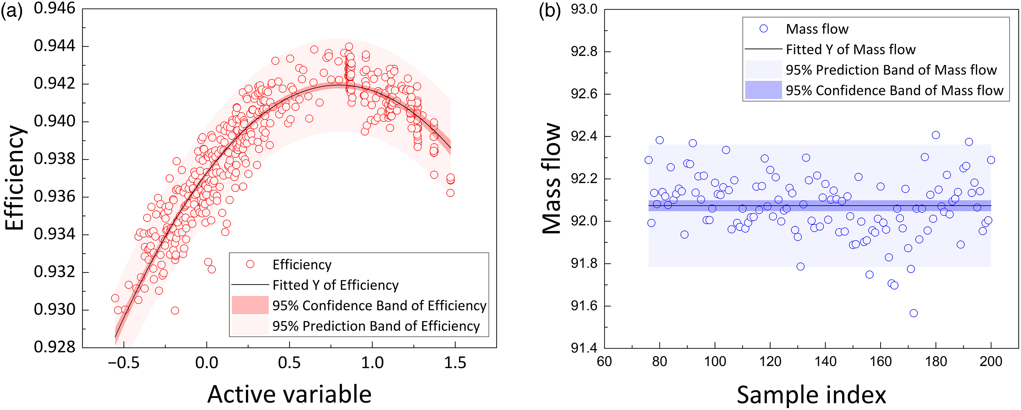
The best value point of this function was found to be 0.82, which corresponded to the highest efficiency of 94.21%. As a result, the value of 0.82 was set as the final aimed value of M1x in Equation (17), along with the desired value of the mass flow, to solve the indefinite equation group using the abovementioned method. The results of the optimized fan after adjusting the aim value are presented in Table 2.

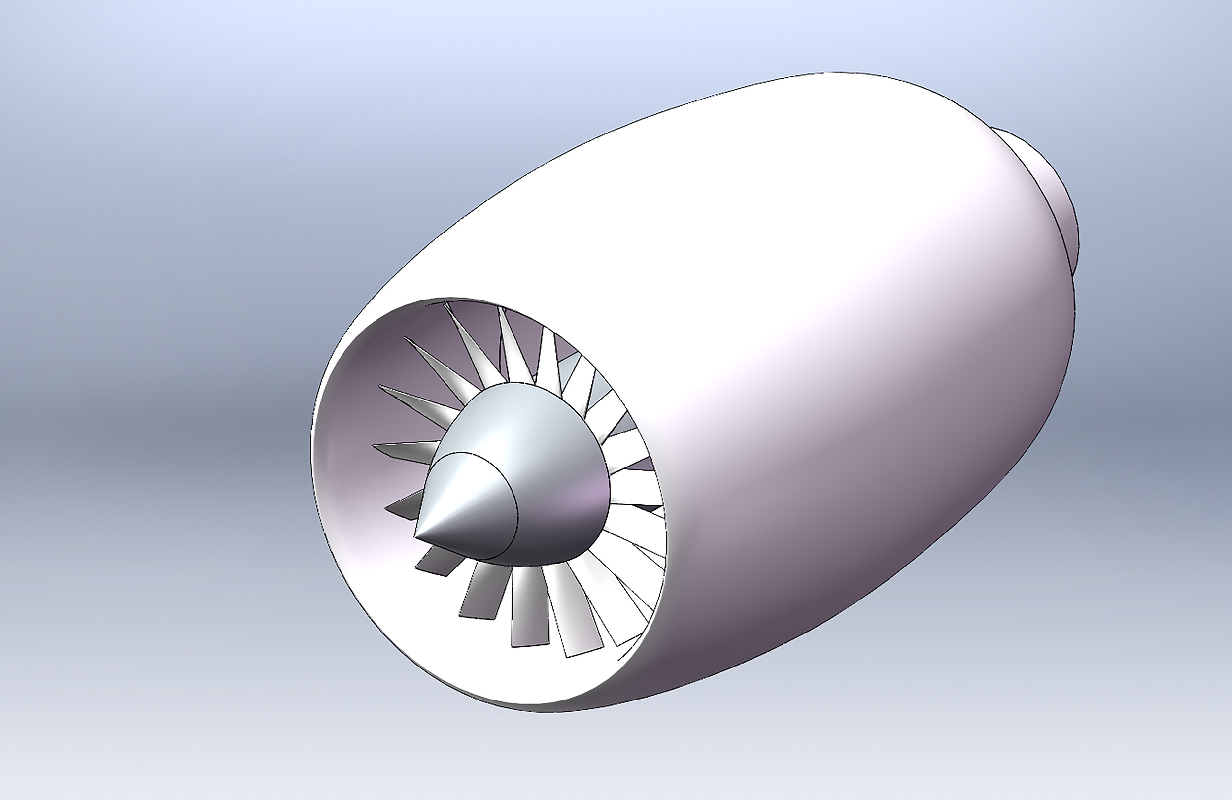
Finally, the blade design with the highest efficiency was chosen as the optimal design, with an adiabatic efficiency of 0.944, mass flow of 92.164, and pressure ratio of 1.203. The primary parameters of the optimized fan are presented in Table 3. Additionally, the blade shape parameters obtained from the optimization process are used to generate a profile file by recalling a customized Multall solver, which includes the 3D coordinates of the stator and rotor. Matlab codes are then used to convert the profile file into a format that can be used in Solidworks software. The resulting 3D model of the optimized ducted fan is presented in Figure 15.

Figure 15.

3D model of the optimized ducted fan with 18 rotors and 4 stators.