
Introduction
Endwall losses are generated by dissipation in the endwall boundary layers and mixing processes. In particular, significant mixing loss may be produced by the secondary flows, which are generated as the non-uniform inlet flow is turned through the blade row.
Of the many aerodynamic and design factors that can influence endwall loss in turbomachinery flows, this paper focuses on the impact of inlet conditions. This sensitivity is of practical importance since the actual boundary conditions inside a machine are unlikely to be known accurately, therefore robust design strategies must be adopted.
This study considers linear cascades with steady inflow, which represent a constrained sub-section of the turbine design space. Nonetheless cascades reproduce many of the underlying physical effects observed in annular turbines and have furthered understanding of the basic problem, as illustrated by the reviews of Sieverding (1985) and Langston (2001). Most experimental cascades operate with an inlet endwall boundary layer formed naturally on the internal upstream walls of the wind-tunnel. Multi-stage inlet flows are more complex due to secondary flows convecting from upstream blade rows and endwall boundary layer skew, and this can lead to additional losses (e.g. Denton and Pullan, 2012). This paper does not examine these effects, rather it attempts to understand the sensitivity of endwall loss to inlet boundary layer thickness for a simple, collinear turbulent profile.
Several authors have examined the effects of inlet boundary layer thickness on cascade loss by installing steps or bleed slots upstream of the test section. Reviewing data from several cascades, Sharma and Butler (1986) argued that the net mass-averaged endwall loss is approximately independent of the inlet boundary layer thickness. Similar observations have been made by other authors (e.g. Hodson and Dominy, 1987), but there are some notable exceptions. For example, de la Rosa Blanco et al. (2003) examined two low pressure turbine blades with identical flow angles but different blade thickness. Increasing the size of the turbulent inlet boundary layer, they found that the endwall loss increased for both blades but more rapidly for the thinner blade. This result illustrates a key finding of the current study, namely that the impact of inlet conditions on endwall loss depends on the design of the blade itself.
The following section describes a computational study of parametric cascade designs. Subsequent sections discuss the impact of inlet boundary layer thickness on endwall loss, the loss mechanisms that drive the sensitivity, and the ability of classical secondary flow theory to model the sensitivity observed.
Numerical methods
Cascade designs
The cascade geometries considered in this paper are taken from the parametric study of Coull (2017). As summarised in Table 1, these 150+ designs cover a large range of flow angles and blade thickness, with different suction surface loading styles (diffusion factor and peak suction location). The previous study considered a constant inlet boundary layer thickness
Table 1.
Cascade design parameters.
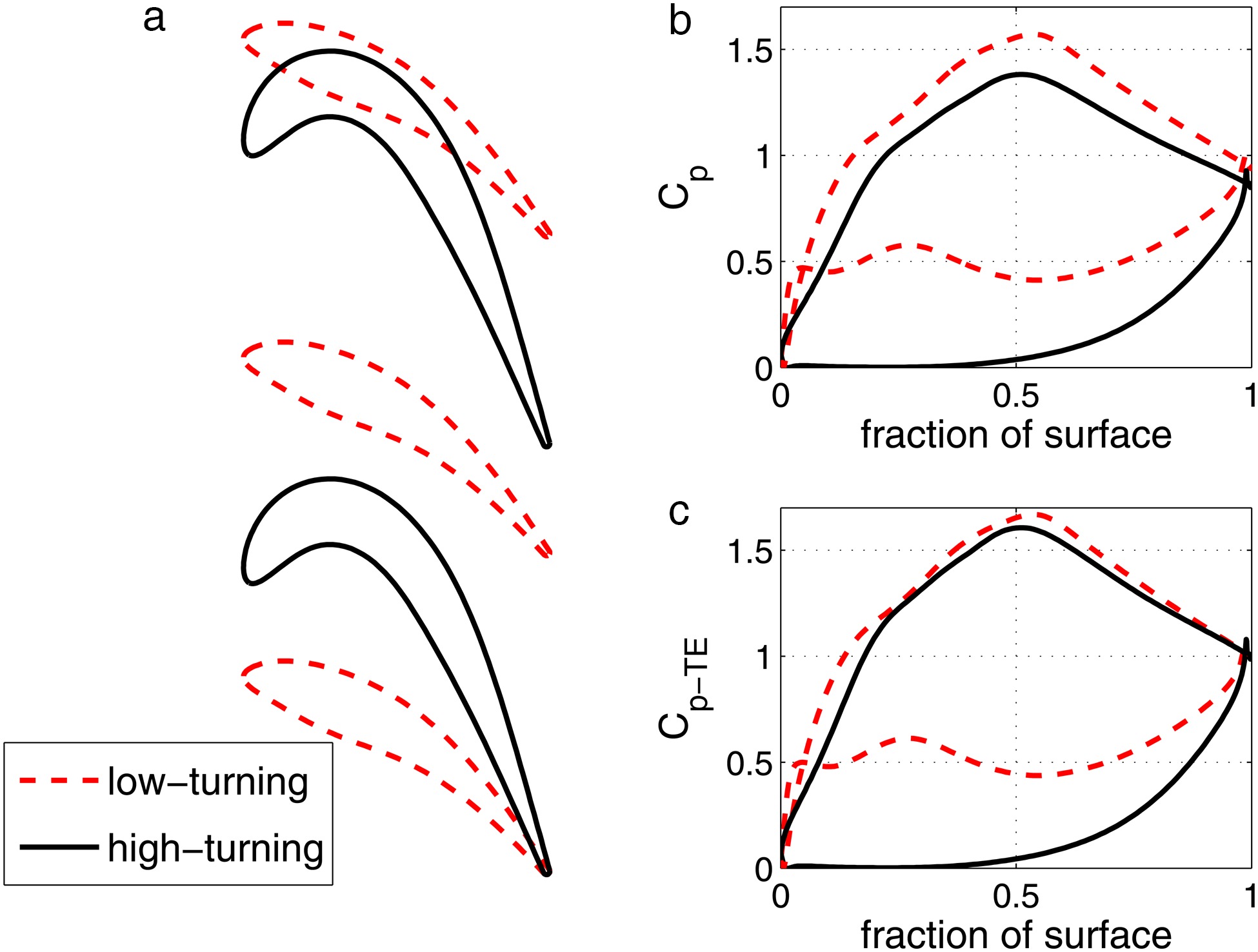
For illustrative purposes, the behaviour of two designs will be described in detail: a low-turning design (
Meshing and CFD
Automated meshing is performed using an optimiser (Coull, 2017) built around the Rolls-Royce PADRAM code (Shahpar and Lapworth, 2003), which combines a blade O-mesh with multi-block passage H-meshes. A maximum
Steady RANS calculations are performed with the Rolls-Royce in-house solver HYDRA. The spatial discretization is based on an upwind edge-based finite volume scheme and is second-order accurate (Moinier and Giles, 1998). Calculations are performed using the two-equation Shear-Stress-Transport turbulence model, with fully-turbulent boundary layers. A half-passage domain is used for each cascade, with an inviscid wall at midspan to provide symmetry. The inlet is located at a distance of
To assess the accuracy of the CFD, calculations are performed for experimental cascade studies (Hodson and Dominy, 1987; Gregory-Smith et al., 1988; de la Rosa Blanco et al., 2003). Figure 2 compares measured and calculated endwall total pressure loss coefficients; the average error is less than 10%, which is deemed to be acceptable.
Figure 2.
Experimental Validation (Hodson and Dominy, 1987; Gregory-Smith et al., 1988; de la Rosa Blanco et al., 2003).

Loss coefficients
This paper considers entropy loss coefficients which give a measure of lost work (Denton, 1993). The general expression for entropy loss coefficient is:
where s is the specific entropy, h is the specific enthalpy and T is the static temperature. This paper considers the mixed-out entropy at the outlet plane
The term
The two-dimensional profile loss is calculated using only the midspan conditions for the inlet and dynamic references:
The endwall loss coefficient
The passage and profile loss coefficients in Equations 2 and 3 have subtly different denominators, which allows for the fact that the two-dimensional losses at each spanwise height will scale with the local dynamic conditions. In the limit of extremely thick inlet boundary layers, significant portions of the blade span will have lower freestream velocity than the midspan and will therefore generate less entropy. Integrated up the span, the profile loss contribution therefore scales with the mass-averaged dynamic conditions, which is accounted for by the switch of dynamic reference between Equations 2 and 3.
Endwall loss sensitivity
Vorticity amplification factor
In order to quantify the secondary flow characteristics of different cascades, Coull (2017) defined a vorticity “Amplification Factor” using the classical theory of Marsh (1976). This parameter is a measure of the area-average secondary vorticity
where p is the pitch,
The integral in Equation 7 is performed over the blade in a similar manner to circulation. The Amplification Factor
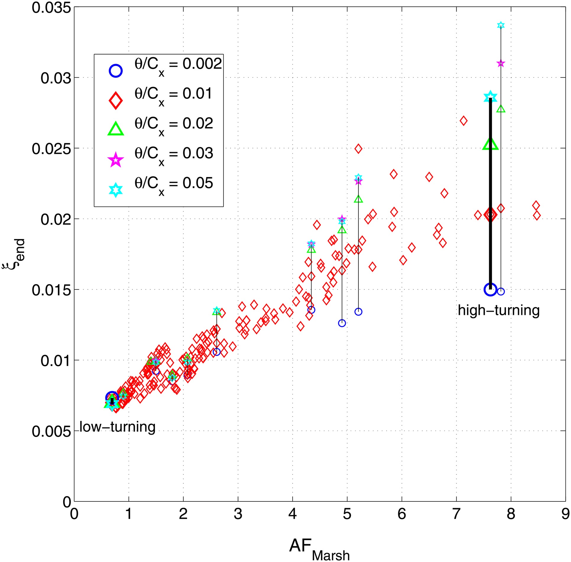
Figure 3 shows the relationship between
Figure 3.
Endwall Loss vs. Vorticity Amplification Factor (Equation 5), with varying inlet boundary layer thickness.
Background dissipation and secondary-flow-induced-loss
A portion of the endwall loss in Figure 3 is generated by viscous shear in the boundary layers on the endwall surface (inside the blade passage and on the platforms upstream and downstream of the blade row). This component of loss is quantified by calculating the “Background Dissipation” loss,
The Dissipation Coefficient
Provided the assumption of constant
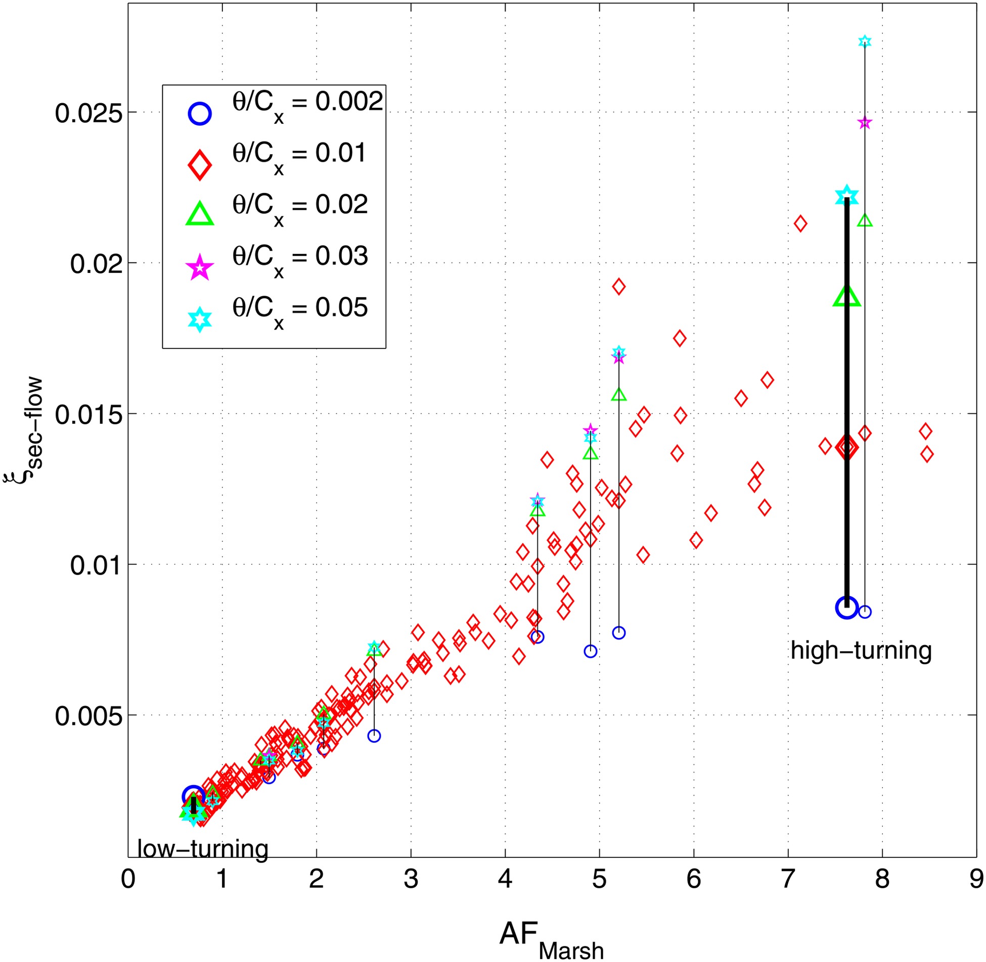
The remaining component of endwall loss is generated by the secondary flows and associated mixing processes:
This definition includes the losses associated with the mixing-out of the non-uniform inlet flow in addition to those directly associated with the secondary flow; in practice it is difficult to separate these effects.
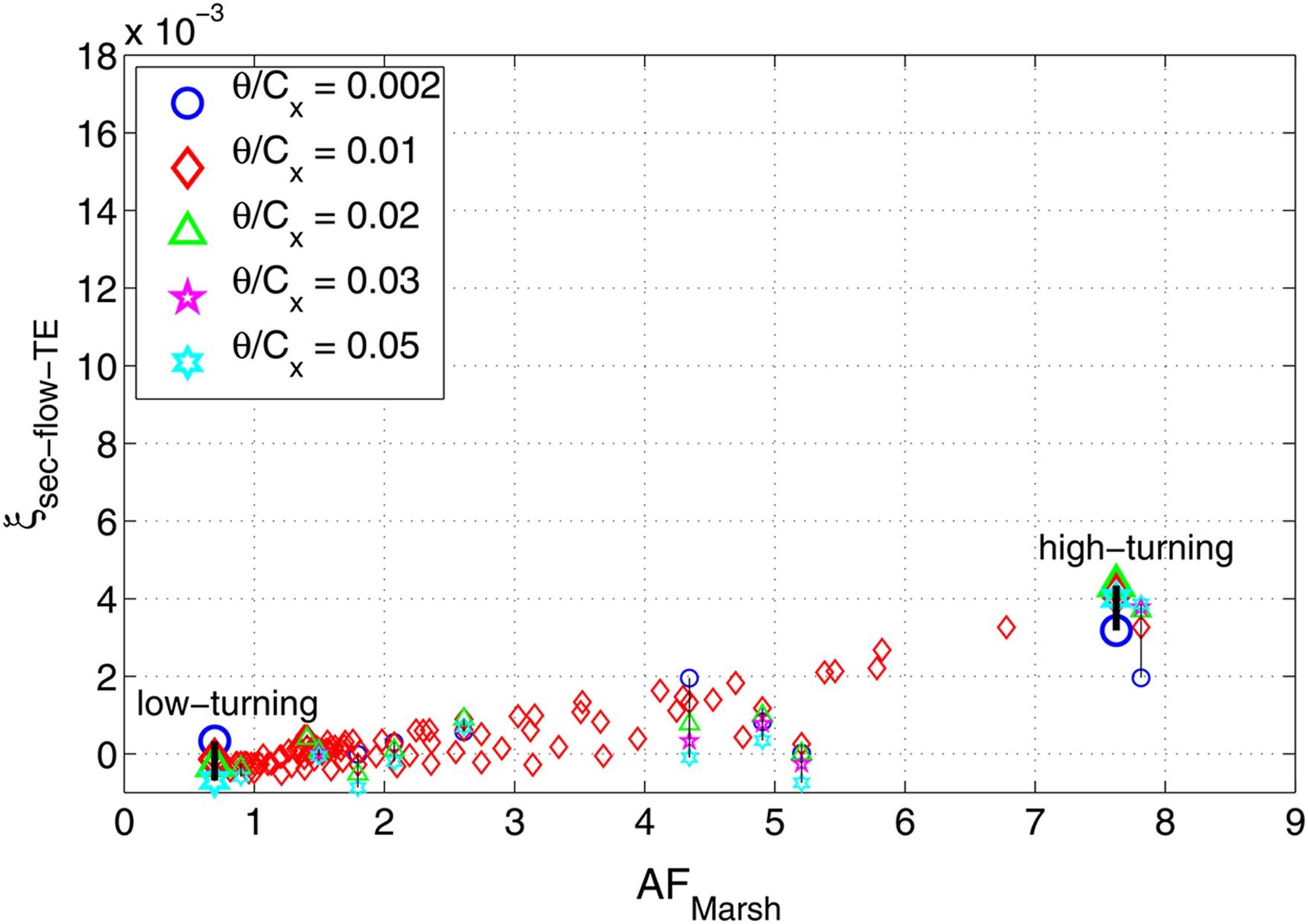
Figure 4 plots the Secondary-Flow-Induced Loss
Previous experimental results
The current results shed some light onto the apparent contradictions in the literature regarding sensitivity to inlet conditions. Figure 5 presents net endwall losses against Amplification Factor (Equation 5) for four cascade designs where the geometry was available. The endwall losses have been re-scaled to match the aspect ratio used in the current study
Figure 5.
Endwall loss vs. Amplification Factor for experimental cases with turbulent inlet boundary layers (Hodson and Dominy, 1987; Gregory-Smith et al., 1988; de la Rosa Blanco et al., 2003).
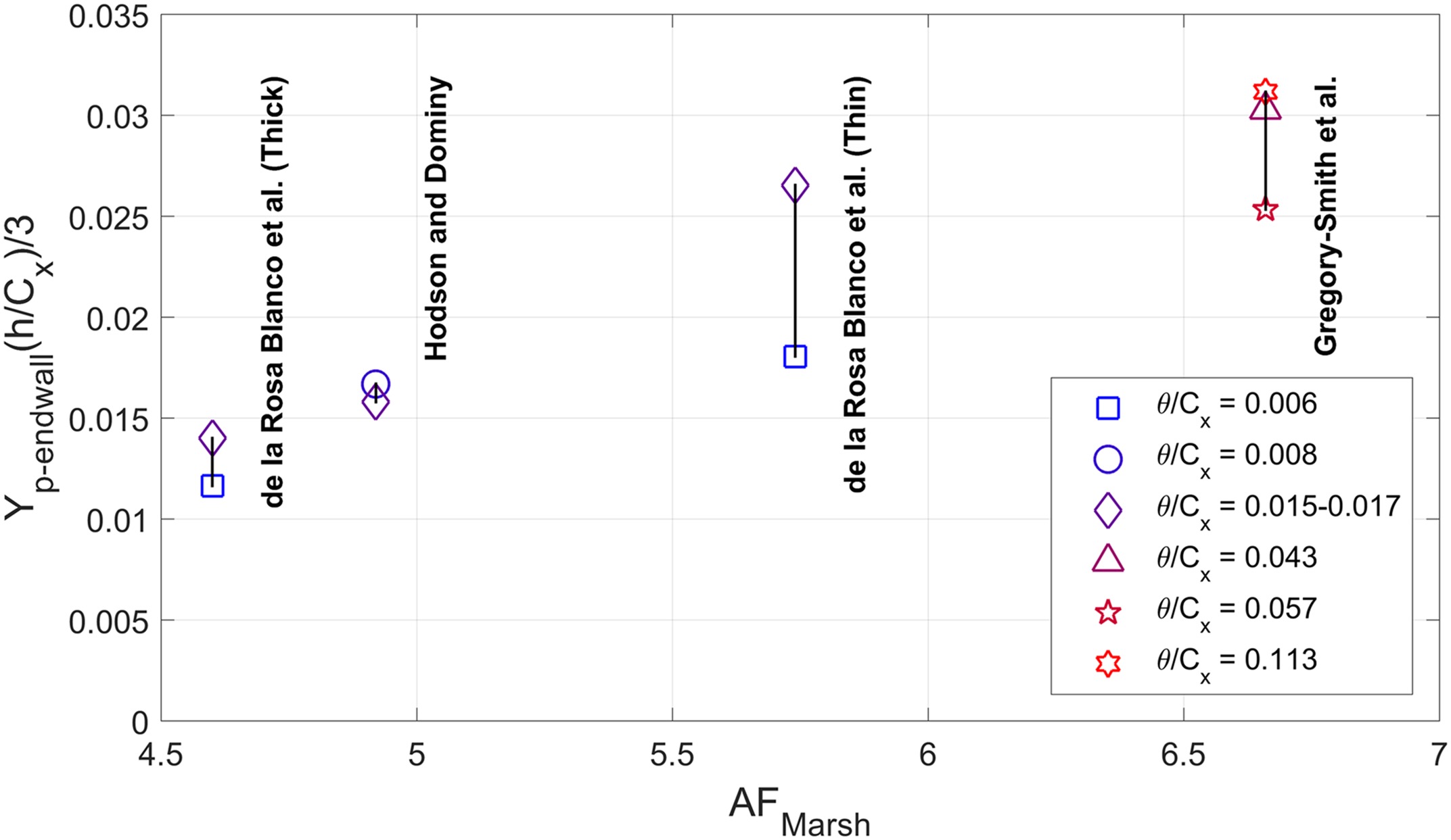
One may conclude that the sensitivity to inlet conditions is driven by the secondary flow, which can be characterised by the Amplification Factor. The remainder of this paper seeks to understand the physical mechanisms that determine this sensitivity in more detail.
Secondary-flow-induced loss mechanisms
This section discusses the three key loss mechanisms that compose the Secondary-Flow-Induced loss
(1) The interaction of secondary flows with blade surface boundary layers;
(2) The dissipation of Secondary Kinetic Energy (SKE);
(3) The mixing-out of Streamwise Momentum Deficits, e.g. regions of low total pressure.
Directly separating the above mechanisms is challenging, even in a CFD calculation. Instead their role is inferred by examining the flow field at the trailing edge plane
Losses inside the passage
Some of the loss generated by the secondary flow occurs upstream of the trailing edge plane, including interaction with blade surface boundary layers (1, above), and partial mixing-out of SKE (2) and Streamwise Momentum Deficits (3). The resultant in-passage loss has been quantified by calculating the mass-averaged secondary-flow-induced loss at the trailing edge plane:
Here
Secondary kinetic energy (SKE)
The secondary velocities are by definition normal to the primary flow direction, which is determined by the midspan flow angle at each pitchwise location, as for example defined by (Denton and Pullan, 2012). The importance of this definition will be demonstrated in “Secondary flow velocities and SKE” below. The losses associated with the mixing-out of SKE downstream of the trailing edge have been estimated by considering localised, constant-pressure mixing. If the secondary velocity is dissipated, the total pressure will drop such that:
where
where R is the gas constant. An SKE loss coefficient is then calculated using the mass-averaged entropy increase
This definition does not include any mixing-out between adjacent fluid particles and only includes the loss that is directly associated with the SKE.
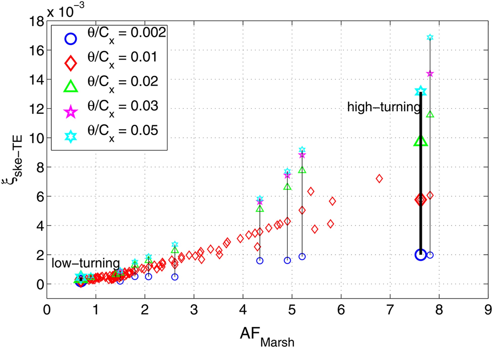
The resultant SKE losses have been presented against the Amplification Factor in Figure 7. For low-
Streamwise momentum deficits
The final component of mixing loss occurs due to the mixing of unlike streams (Denton, 1993). Considering a control volume downstream of the trailing edge, this mixing loss is driven by the streamwise momentum deficits of the flow leaving the cascade. Such deficits arise due to the convection and distortion of the (low-total-pressure) inlet boundary layer fluid, the development of losses in the passage, and from regions of significant under- and over-turning induced by the secondary flow.
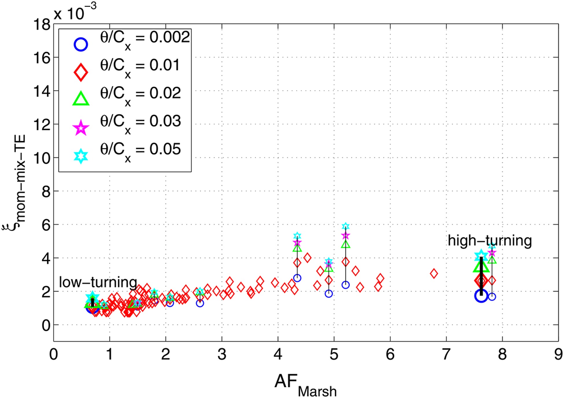
From the trailing edge data, a constant-area mixing calculation is performed and the endwall contribution to the mixing loss
As shown in Figure 8 this component of loss rises approximately linearly with the Amplification Factor, and has relatively low sensitivity to the inlet boundary layer thickness compared to the SKE loss. For the low-turning design the streamwise momentum deficit loss is small (∼0.0015) and is approximately equal to the overall secondary-flow-induced loss for this design (Figure 4). For the high-turning design, the momentum deficit loss is slightly larger but represents a smaller fraction of the overall loss.
From the relative magnitude of each term in Figures 6–8, it is clear that it is largely the Secondary Kinetic Energy (Figure 7) that determines the sensitivity to inlet conditions. The results also reveal a switch in mechanism for the secondary-flow-induced loss: low-turning designs are dominated by the mixing-out of Streamwise Momentum Deficits; while for higher-turning designs the SKE tends to dominate. An extreme example of this behaviour is a zero-turning duct with no blades, no secondary flow generation and thus only loss from the mixing of Streamwise Momentum Deficits.
Modelling secondary flow
Having demonstrated that SKE dominates the sensitivity of endwall loss to inlet conditions, the analysis now applies a theoretical model to highlight the underlying physical mechanisms.
Vorticity amplification theory
The prediction of secondary flows was studied intensely in the early years of turbomachinery research. “Classical” theories focused on the analytical prediction of secondary vorticity and velocity, as reviewed by Horlock and Lakshminarayana (1973). Assuming inviscid flow, these methods predict the exit streamwise vorticity by considering the convection and reorientation of the inlet boundary layer vorticity as it convects through the blade row. For incompressible flow, Hawthorne (1955) used a vortex-filament analysis and applied Helmholtz’s theorems, while Came and Marsh (1974) presented an alternative approach based on Kelvin’s Circulation theorem. Both approaches give the same expression for the distributed vorticity associated with the passage vortex and bulk secondary flow.
This paper applies the method of Marsh (1976) who extended the circulation analysis to include compressibility. The method assumes that the flow through the blade row is parallel to the endwall, without streamtube contraction or twist. At each spanwise height the ratio of outlet-streamwise vorticity to the inlet-boundary layer vorticity is given by:
This equation has been applied to each case using the radial-averaged inlet conditions from the CFD calculations (total pressure, static pressure and flow angle) and area-averaged outlet pressure. Figure 9 illustrates the vorticity calculations for the low (a–f) and high (g–l) turning designs with two different inlet conditions.
Figure 9.
Vorticity Calculations for the low-turning (top row) and high-turning (bottom row) designs: (a, g): inlet velocity; (b, h): inlet vorticity; (c, i): isentropic velocity ratio; (d, j): vorticity ratio (Equation 16); (e, k): calculated exit streamwise vorticity; (f, l): CFD streamwise vorticity at the trailing edge plane.
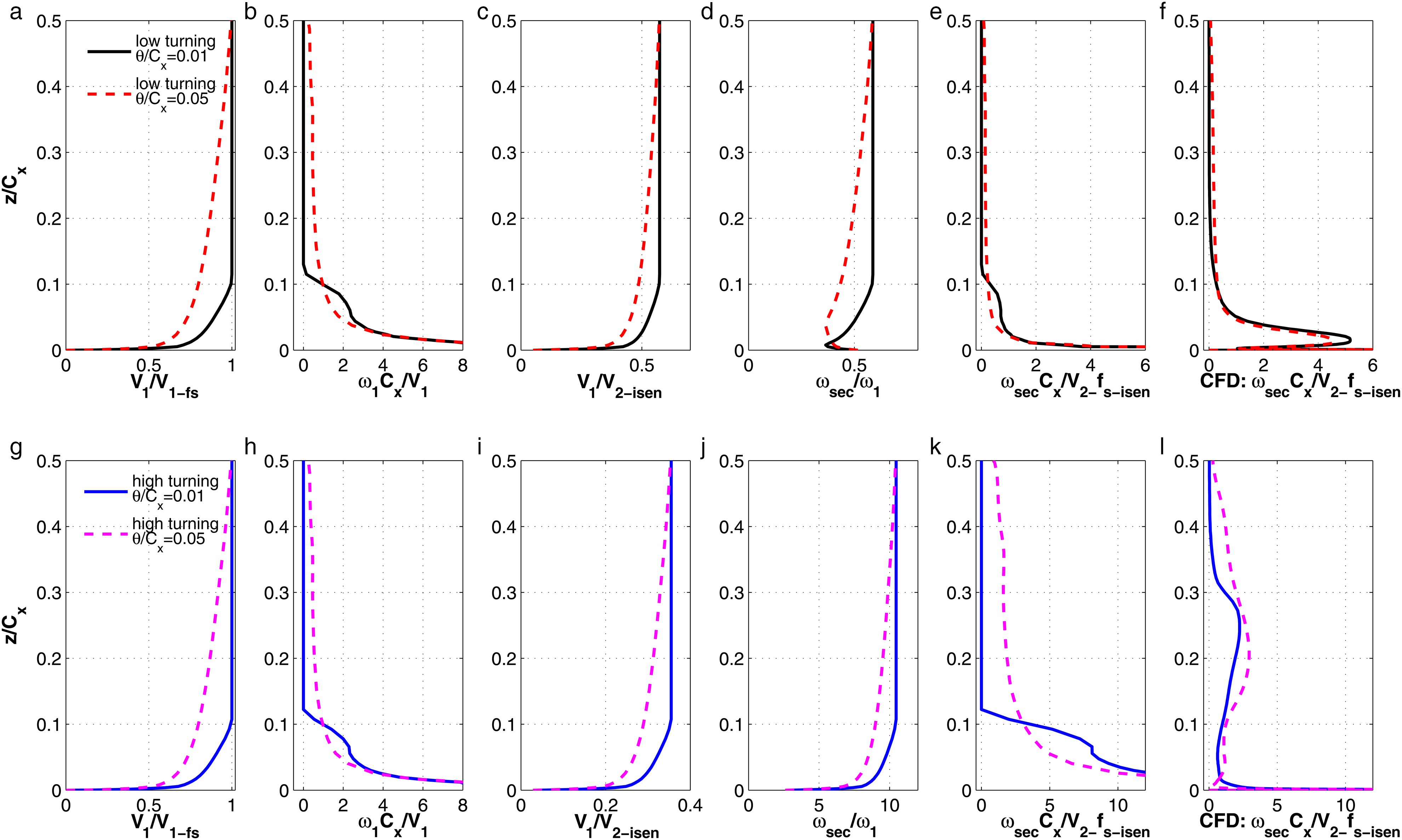
Figure 9a and g show the normalised inlet velocity profiles; Figure 9b and h show the associated boundary layer vorticity. By definition the area-averaged inlet vorticity is independent of the boundary layer thickness. The thicker boundary layer has higher vorticity in the “outer” region of the span
The terms in Equation 16 are calculated at each height. The velocity ratio
The calculated outlet streamwise vorticity is presented in Figure 9e and k. For each design, the overall pattern of outlet vorticity largely follows that of the inlet vorticity. Thicker boundary layers cause higher levels of vorticity in the outer region
For comparison, Figure 9f and l present equivalent data from the trailing edge plane of the CFD calculations: streamwise vorticity of the same sign as the passage vortex has been mass-averaged in the pitchwise direction. For the low-turning design the model (Figure 9e) and CFD (Figure 9f) show reasonable agreement. As the boundary layer thickness is increased, the two plots show an increase in vorticity in the outer region
Secondary flow velocities and SKE
The secondary velocities associated with the predicted vorticity field of the Marsh model are calculated via a streamfunction
where
It is worthwhile to highlight the importance of the definition of the primary flow direction. For the low-turning design, Figure 10a shows the Marsh model prediction of secondary flow streamlines with contours of SKE loss (Equation 14). Figure 10b shows the equivalent CFD data at the trailing edge plane, with the primary flow angle defined as the mass-averaged value
Figure 10.
Secondary Flow Definitions for the low-turning design, θ / C x = 0.01
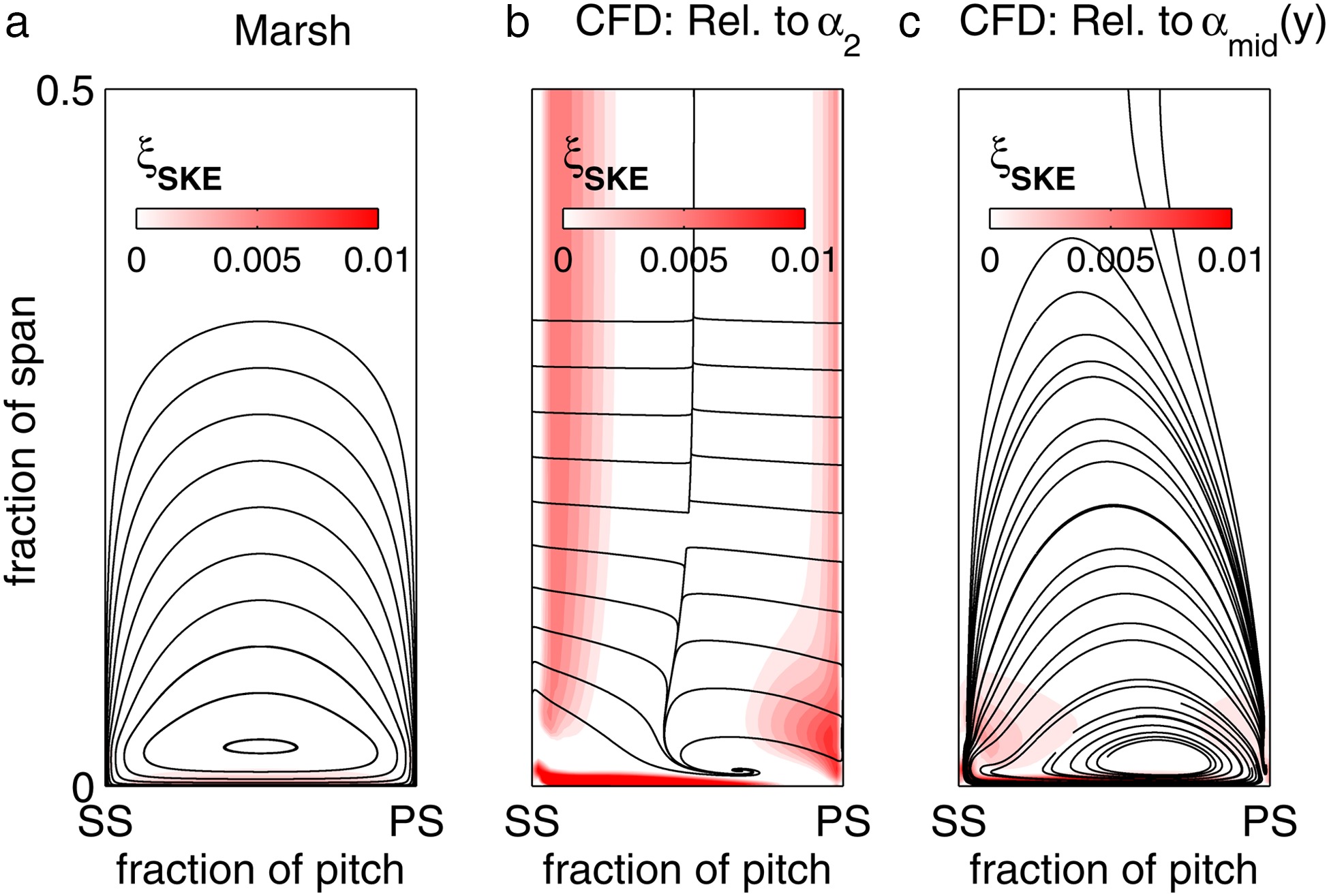
Figure 11 compares the Marsh predictions to the CFD results for the low and high-turning cascades, with two inlet boundary layer thicknesses. The lack of streamtube twist in the model always leads to symmetric solutions. For the high-turning CFD results (Figure 11c(ii) and d(ii)) there is significant streamtube twist and asymmetry. In particular, the vortex core has moved towards the blade suction surface inducing high SKE in this region. Despite these differences the Marsh model does a reasonable job of capturing the overall pattern of the secondary flow and the size of the passage vortex. The order-of-magnitude increase in SKE between the low and high-turning designs is captured (note the different scales); the model also predicts the higher SKE for the thicker inlet boundary layer, in particular for the high-turning design (Figure 11c and d). The Marsh model highlights the importance of the distribution of secondary vorticity within the passage. As the boundary layer thickness increases, the average vorticity level remains approximately constant but the vorticity becomes more dispersed within the passage (Figure 9e and k). This dispersed vorticity field results in larger secondary flow structures with higher overall secondary kinetic energy.
Figure 11.
Secondary-Flow Streamlines and SKE: Marsh model and CFD results; pitchwise direction is normal to the exit flow angle.

For all of the cases studied, Figure 12 compares the SKE loss from the Marsh model with the CFD values extracted at the trailing edge plane. Reasonably good agreement is found for most designs. For the high-turning design the modelled values are higher but this likely reflects the increased dissipation of SKE within the blade passage for this design (Figure 6).
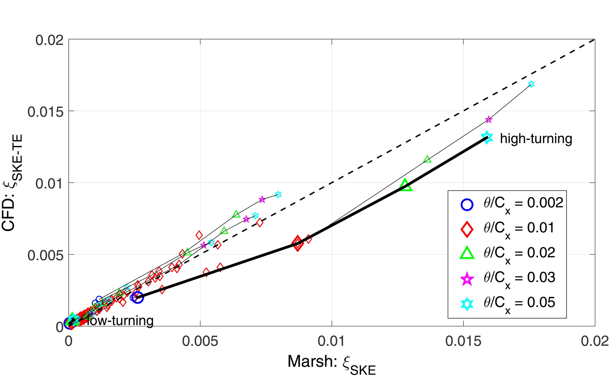
Figure 13 presents the SKE loss for the Marsh model plotted against the Amplification Factor, which is in close agreement to the CFD data in Figure 7. The trends in Figure 13 re-iterate the two factors determining SKE:
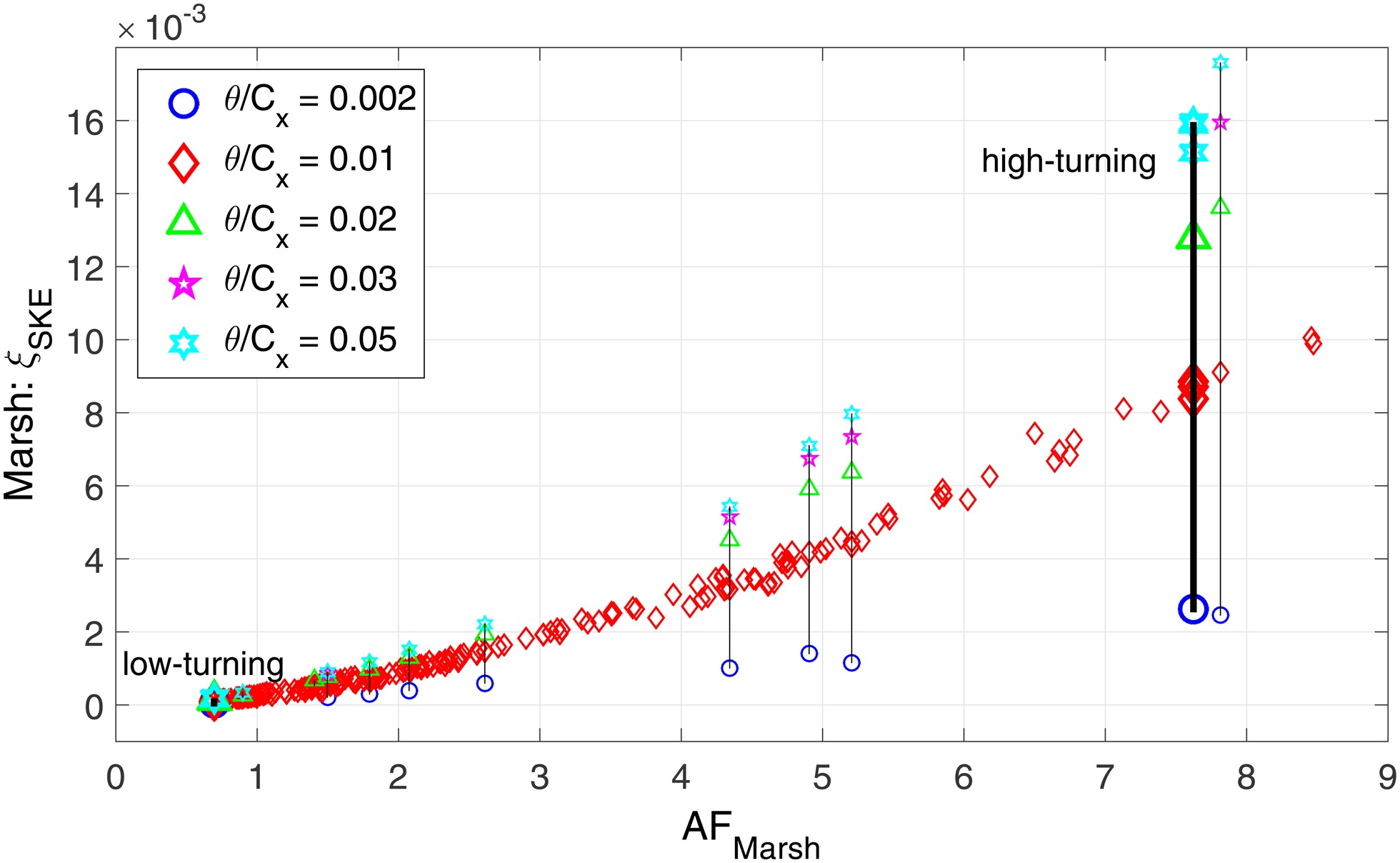
The average value of secondary vorticity
The distribution of vorticity within the passage, which is determined by the inlet boundary layer. Thin inlet boundary layers tend to produce secondary flows structures that remain close to the endwall (e.g. Figure 11c). Thickening the inlet boundary layer displaces vorticity away from the endwall, tending to generate larger secondary flow structures (e.g. Figure 11d). Such larger vortex structures tend to have higher associated SKE (e.g. Clark et al., 2016), leading to an increase in loss.
For designs with high
Conclusions
The sensitivity of endwall loss to inlet conditions is design-dependent, and is largely driven by the component of loss associated with the secondary flow and associated mixing processes.
The Secondary-Flow-Induced loss can be characterised by an Amplification Factor
The sensitivity is primarily driven by the dissipation of Secondary Kinetic Energy (SKE). To a first order, the SKE generated by a turbine cascade is governed by the average level of streamwise vorticity
Designs with low Amplification Factor
The variations in SKE can be captured using a simple model based on the inviscid vorticity calculation of Marsh (1976) and the streamfunction approach of Squire and Winter (1951). A similar approach could be used to perform sensitivity assessments in the preliminary stage of design, and could be readily extended to engine-realistic boundary conditions.
Nomenclature
Symbols
Area
Vorticity Amplification Factor (Equation 5)
Aspect Ratio
Dissipation Coefficient
Specific Heat Capacity (isobaric)
Pressure Coefficient
Pressure Coefficient
Axial Chord
Specific Enthalpy
Span
Mass flow rate
Mach number
Pitch
Static and Total Pressure
Axial Chord Reynolds number
Specific Entropy
Distance along Surface
Trailing Edge Thickness
Temperature
Non-Dimensional Surface Transit Time
Velocity
Axial Distance
Pitchwise Distance
Total Pressure Loss Coefficient
Spanwise Distance
Zweifel Lift Coefficient
Flow Angle
Specific Heat Ratio
Inlet Boundary Layer Displacement Thickness
Inlet Boundary Layer Momentum Thickness
Kinematic Viscosity
Entropy Loss Coefficient
Density
Vorticity
Subscripts and Abbreviations
0
Stagnation
1, 2
Row Inlet and Outlet
Background Endwall Boundary Layer Dissipation
Diffusion Factor
Boundary layer edge
Isentropic
Leading Edge
Midspan (Profile)
Mixed-Out (Constant-Area)
Streamwise Momentum Mixing Loss
Normal to Primary-Flow and Spanwise directions
Pressure Surface
Peak Suction Location (fraction of surface length)
sec-flow
Secondary-Flow-Induced Loss
Secondary Kinetic Energy
Suction Surface
Trailing Edge