
Introduction
The current industry practice for blade design initially involves combining numerical and experimental techniques to determine the heat transfer coefficient levels obtained by a particular cooling system. These levels are then often passed to a separate team which applies them to a full blade stress model to determine if a particular blade design has adequate life (Cunha, 2006; Friedrichs, 2012). This process can be time consuming and expensive due to the multiple full analyses that must be undertaken, with each change in cooling design requiring a full re-analysis.
The aim of the present research is to improve this process by obtaining an enhanced understanding of the influence of changes to the cooling system on the stress distribution directly, rather than continually altering a complete cooling model of a blade until the required blade life is reached.
The focus of this work was to investigate the convective parameters responsible for the temperature field and also their net effect on the stress field, obtained from an elastic stress distribution, which influences blade life.
The intent was that this study could be used to directly improve the cooling performance of a blade design through the variation of HTCs in different regions, either by geometric or convective changes, as well as to assess the effect of uncertainty in the HTC levels used in the modelling process on the temperature and blade life.
The method used here isolates a single cooling system, and uses a thermal FEA model with HTC and temperature boundary conditions to provide a metal temperature distribution, which is then used in a stress analysis.
Using an imported FEA temperature distribution significantly reduces the time taken for each simulation and also allows for the effect of altering HTC levels on different surfaces to be directly modelled, rather than using a full conjugate CFD simulation where the causes of any changes in stress distribution could be difficult to isolate, whilst also taking longer to run.
Methodology
The method involves a number of stages which are illustrated in Figure 1.
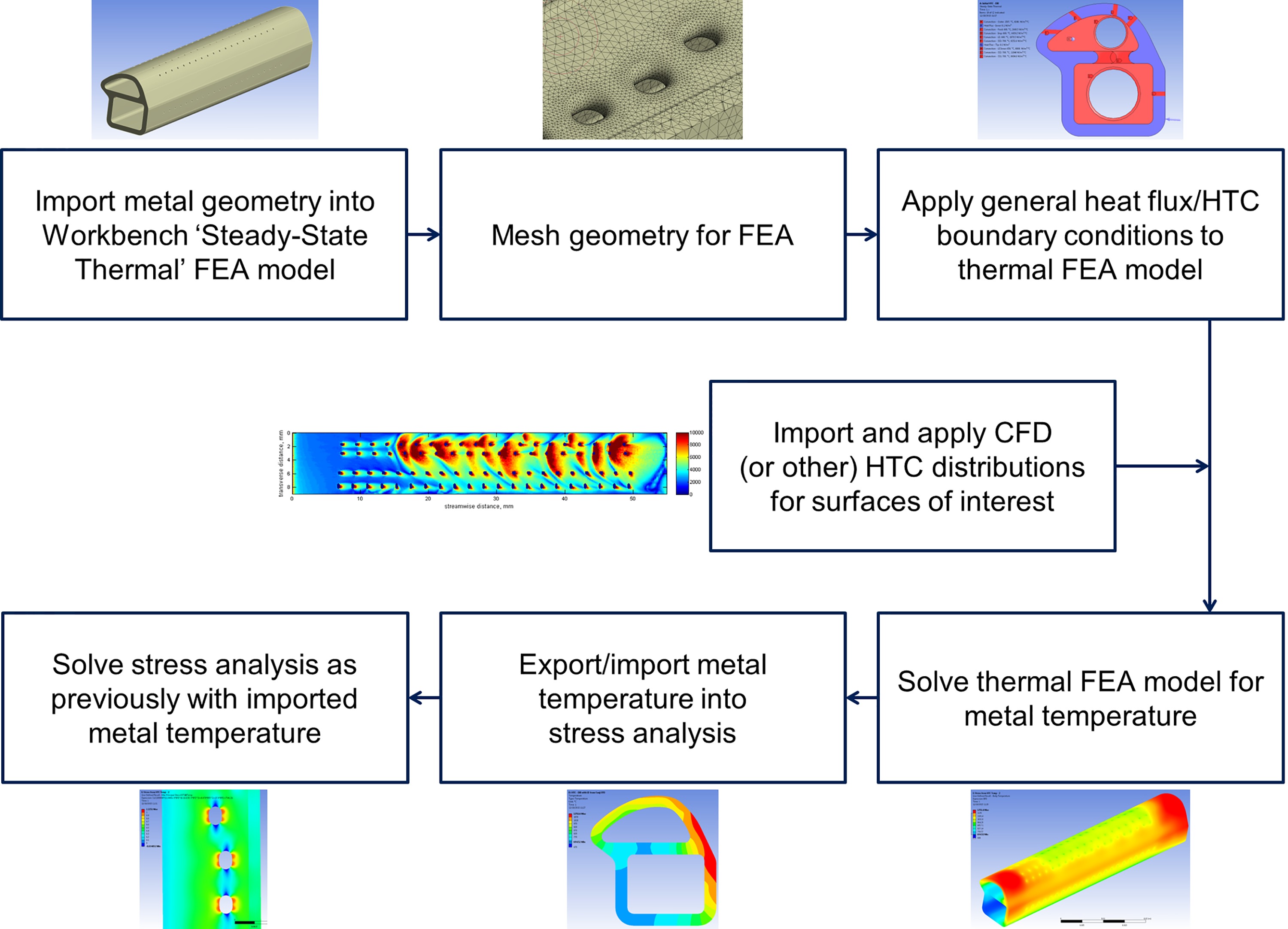
Initially the required geometry is produced using CAD software and imported into ANSYS Workbench. A ‘Steady-State Thermal’ FEA model is then created using this geometry. Following this, the geometry is meshed using the in-built Ansys Mechanical meshing software. In this paper the geometry analysed as a leading edge impingement system. Such systems can offer high heat transfer levels that are required for the high heat loads found at the leading edge of a turbine blade (Han, 2004; Zuckerman and Lior, 2006). For this particular leading edge geometry a global element size was set, with refinement on the film and impingement hole surfaces. Once meshing has been completed, thermal boundary conditions are applied to the model. In this case, heat flux conditions and HTC with driving gas temperature conditions were used on internal and external surfaces. The boundary conditions can either be specified directly as constant values on each surface or using an imported distribution. For the leading edge internal surface a full distribution from a conjugate CFD simulation was imported and mapped to the relevant surfaces. The thermal model is then solved using the Ansys Mechanical FEA software to give a full, three-dimensional metal temperature distribution. The material properties were set to be representative of a modern turbine blade, using the material Rene N5 which exhibits similar properties (Nickel Dev. Inst., 1995). The full temperature distribution is then analysed, and also exported for use in a stress analysis. A stress analysis is performed using the imported temperature distribution.
The initial metal temperatures from the FEA simulation with imposed heat transfer conditions on the boundaries is imported into the Ansys Mechanical software and mapped onto the solid domain using the imported load tool. Rotation about a rotational axis at an engine representative angle and speed was included to simulate that experienced in an engine. The blade was anchored at a fixed radial displacement, that matched the engine dimensions, on the root surface of the geometry. This boundary condition causes a region with very high stresses near the root of the blade, however this stress concentration was localised and did not affect the area of interest in the central section of the metal. It also closely simulates the actual boundary condition found in the engine, with the fir tree anchoring the blade root to the disk. An elastic stress analysis was then carried out using these conditions.
Thermal simulation details
The finite element simulation requires many different thermal boundary conditions, which in this case are taken from a combination of correlations and other simulations. Figure 2 illustrates the different regions to which thermal boundary conditions were applied.
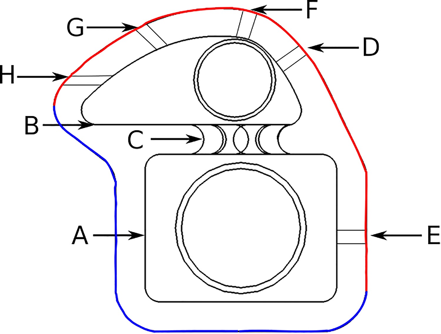
The external surfaces were modelled with a uniform HTC of just over 4000 W/(m2K) and a free stream temperature of approximately 1800 K applied over the leading edge, shown as the red boundary in Figure 2. The remaining external surfaces were modelled as adiabatic, as in a real blade case these would be internal to the blade and therefore not expected to cool this portion of the blade. These are shown as blue in Figure 2.
The internal surfaces were modelled using a constant representative coolant gas temperature for simplicity, and earlier conjugate CFD analysis showed there is relatively insignificant temperature change (less than 3°C) throughout the passage length. The HTCs on the internal surfaces were calculated using the Dittus-Boelter correlation to achieve representative levels for each passage, apart from the leading edge internal surface where a distribution was imported from a conjugate CFD solution. This was undertaken to remain representative of a real system as under the impinging jets there are large spatial variations in HTC.
Details of heat transfer coefficients applied to each internal surface are given in Table 1. These were all calculated using the Dittus-Boelter correlation based on the Reynolds number and hydraulic diameter of the relevant feature.
Results and discussion
Comparison of new method with conjugate CFD
The results obtained using the FEA thermal simulation are compared below to those obtained using a full conjugate CFD solution, in order to verify that the salient features in the temperature and stress distributions are accurately represented.
Temperature distribution
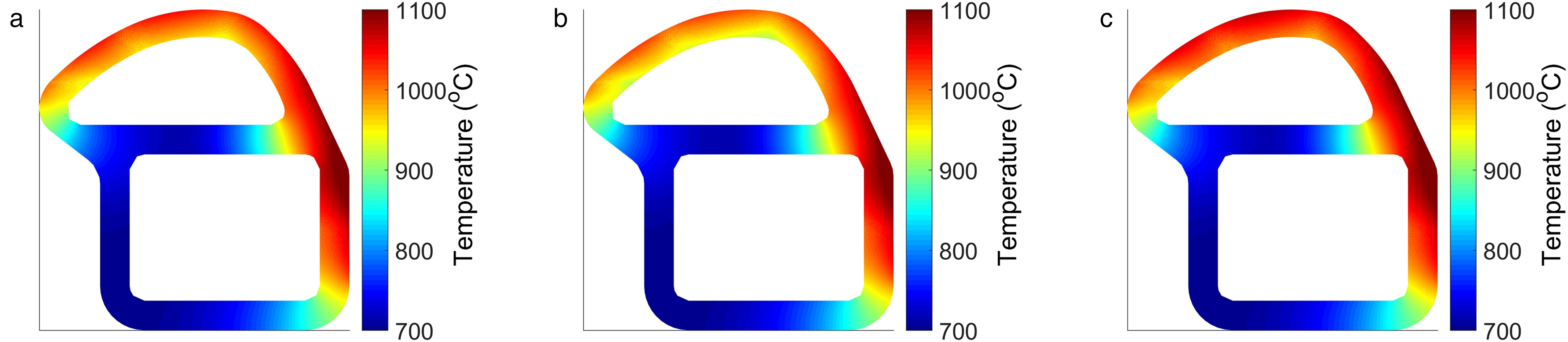
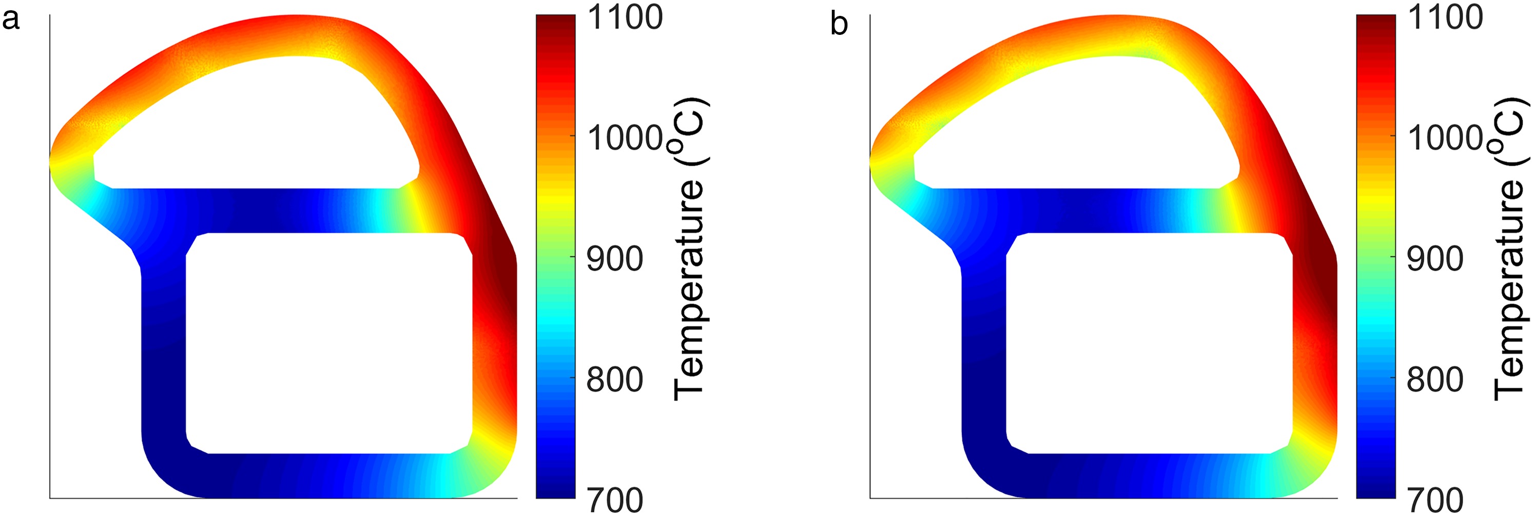
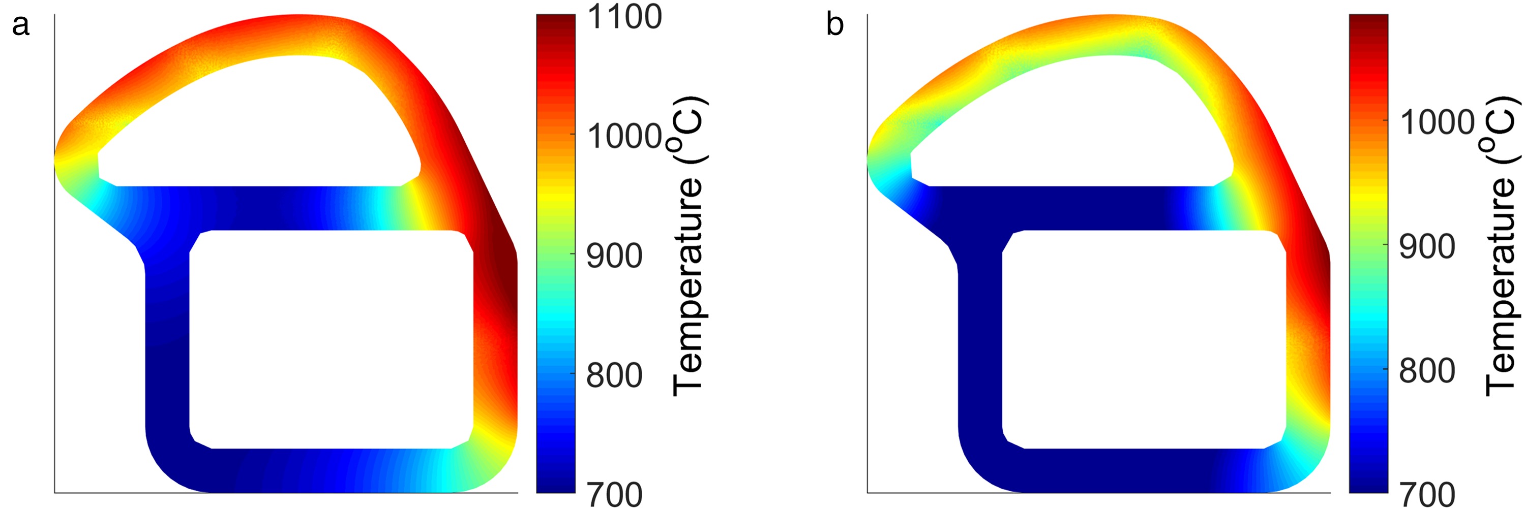
Figure 3 compares the metal temperature distribution from the conjugate CFD to that obtained by the new method as described above.
Figure 3.
Conjugate CFD vs thermal FEA metal temperature comparison: (a) conjugate CFD, (b) thermal FEA.

The general trends in distribution are seen to be similar in both cases with high temperatures around the right hand section of the blade, and considerably lower temperatures in comparison to this under the impingement jets. The lowest temperatures are also found in the web, due to the in-hole cooling effect of the impingement system, and in the feed wall where the adiabatic boundary condition is found. However the conjugate CFD shows consistently lower temperatures than the new method. This is due to the underestimated heat pickup caused by using the Dittus-Boelter correlations. The correlation does not take into account local features, such as separation and reattachment regions, which can significantly raise the heat transfer levels. However, the temperature distribution from the FEA model is close to the conjugate CFD, and maintains the key features of the distribution, such that it is used as a baseline from which relative changes due to HTC adjustments can be assessed.
Stress distribution
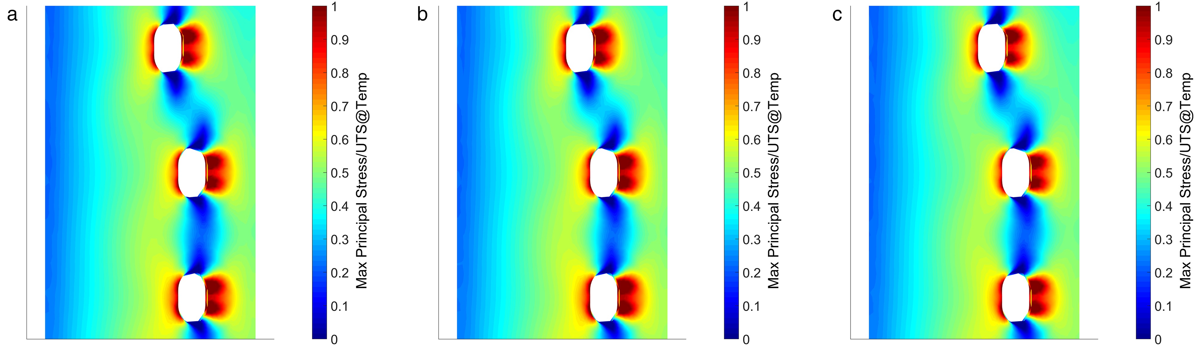
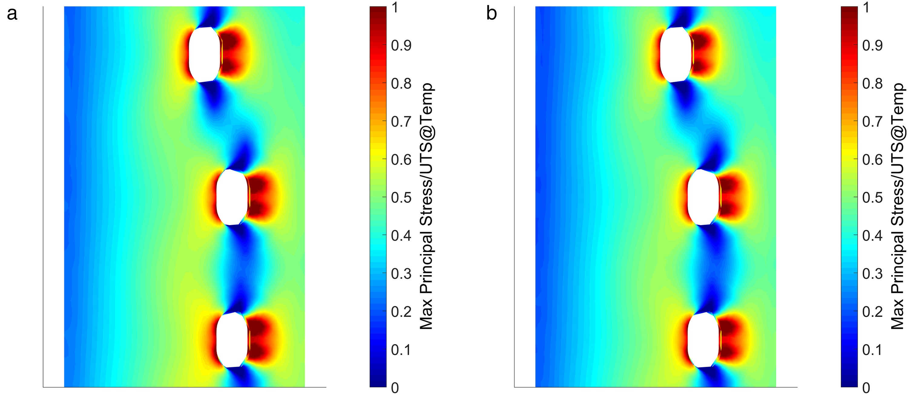
Figure 4 compares the stress distribution from the conjugate CFD to that obtained by the new method. The stress distributions are displayed in the form of maximum principle stress/UTS (ultimate tensile stress) at temperature contours. This metric is used as maximum principal stress is a key driver of blade life, however the material properties change greatly with temperature and this must be taken into account when assessing the stress performance.
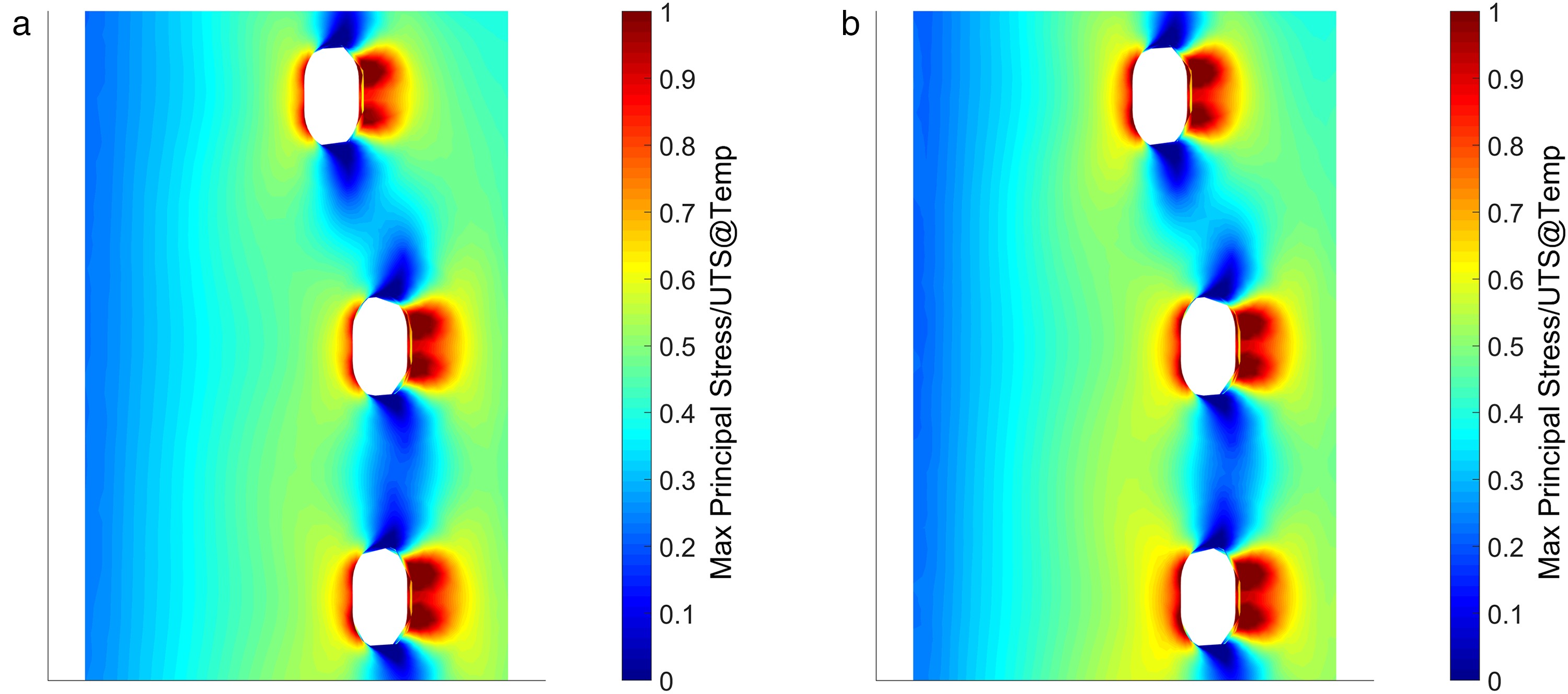
The distributions are seen to be very similar for these two simulations. The stress concentrations around the impingement holes are of similar shape and magnitude while web stress levels further from the holes are also seen to be very well matched.
This confirms that the FEA thermal model with applied HTCs is representative of the fully resolved conjugate simulation, and therefore can be used as a baseline from which to assess the effect of HTC alterations in different regions.
HTC adjustments – influence on temperature
Following the establishment of the method, HTC levels were systematically varied on the different surfaces in order to assess the sensitivity of both metal temperature and stress levels to changes in HTCs. HTCs were varied on the leading edge, web and in-hole areas by ±20%. This level of change was chosen as it is likely to be achievable by improvements in cooling technology whilst remaining realistic. It was judged to be large enough to cause identifiable changes in both temperature and stress distributions if these are reasonably dependent on the HTC levels in the areas which are investigated.
Leading edge
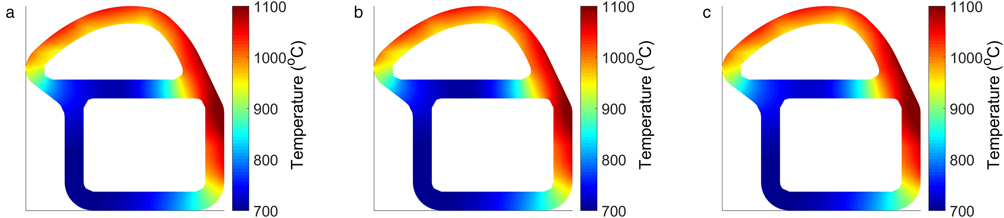
The temperature distributions for the leading edge internal HTC alterations are given in Figure 5. It is clear that the alteration of the leading edge heat transfer levels influences the metal temperature in this region. An increased HTC greatly reduces the temperature while it is increased for a reduction in HTC levels. Other regions of the leading edge model remain unaffected by this change with no differences in temperature observed other than in the leading edge region. This indicates that the leading edge HTC can be altered to obtain a more desirable temperature without impacting the temperature distribution in other regions.
Web
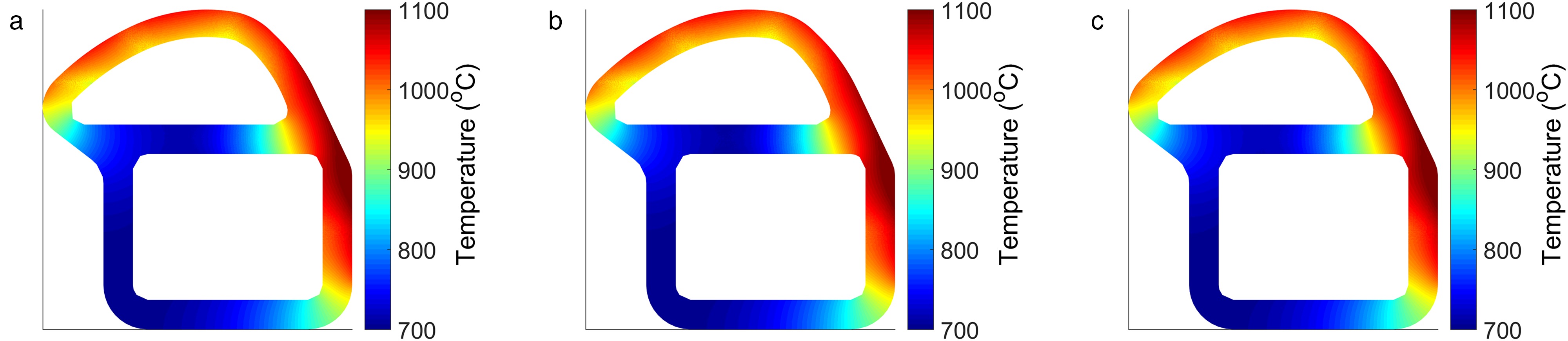
Temperature distributions from the simulations with the web HTC altered are given in Figure 6. The changes in temperature for this case are less prominent than those on the leading edge due to the lower heat fluxes involved, however clear changes are observed. These changes are also in regions of higher stress so are still likely to impact on the stress/UTS at local temperature levels, and therefore blade life. As would be expected the higher HTC levels result in a cooler web with a lower HTC giving a hotter web. However a hotter web is likely to be desirable to reduce stress and increase blade life.
In-hole
Figure 7 shows the temperature distribution’s sensitivity to in-hole HTC levels. The in-hole HTCs are very high, and therefore a significant change in temperature might be expected to occur from this perturbation.
However due to the small surface area over which the coolant acts very little change in temperature distribution is observed in comparison to those resulting from other heat transfer alterations. A small change in web temperature is found, but significantly less than those from the same proportionate changes in HTC on the web.
In summary it is found that alterations to the leading edge and web heat transfer coefficients result in significant changes in temperature distribution, whilst the in-hole HTC alterations do not. This result guided the subsequent research away from a consideration of the in-hole convective HTC. This is significant as the author was aware of forced geometric changes to the hole geometry which would affect this HTC distribution. The changes in temperature distribution are large enough that changes in the stress distribution would be expected. The changes in temperature distribution are isolated in the region in which the HTC is altered.
HTC adjustments – influence on stress
Leading edge
The stress distributions from simulations that use the temperature distributions resulting from the leading edge HTC adjustments are shown in Figure 8.

This figure indicates that there is a small change in the web stress distribution for these cases. It would be expected for there to be lower stress levels in the case with higher LE HTCs as the lower leading edge temperatures would lead to less differential expansion between the web and outer shell. The opposite would be expected for the case with lower LE HTC levels. This is observed to some degree, with stress levels around the impingement holes seen to be slightly lower for the raised HTC case, however the changes appear to be fairly small.
Web
Figure 9 gives the stress distribution with altered web HTCs.

This case only shows very small changes in stress levels for the given alterations. The increased web HTC exhibits slightly higher stress levels, as the colder web results in greater relative expansion of the outer shell to the web. The reverse effect is seen when the web temperature is increased with a decreased HTC level.
In-hole
The stress distributions for adjusted in-hole HTC levels are shown in Figure 10.
Figure 10.
In-hole HTC ±20% - stress distribution: (a) thermal FEA, (b) in-hole +20%, (c) in-hole −20%.
There are no visible differences in these stress distributions. This is expected due to the lack of any significant temperature changes resulting from the in-hole HTC adjustments.
A number of interesting points can be drawn from this section.
It is observed that a 20% change in HTC levels can have a significant impact on metal temperature levels. Alterations in the leading edge HTC have the greatest effect, however in-hole levels have a very limited impact due to the small surface area.
The changes in metal temperature are seen to be isolated in the region in which the HTC is altered, with no indirect effect in other regions of the metal.
Stress levels are seen to be reduced by either increasing the leading edge HTC, or decreasing the web HTC as this reduces the temperature difference between the web and shell and consequently the relative expansion of the shell compared to the web. Visually the changes in stress levels are small, however due to the high dependency of life on these levels they can still be significant.
Combined HTC adjustments
Following the assessment of individual HTC adjustments a simulation was run to obtain a further reduction in stress levels through the combination of multiple adjustments. Due to the isolation of the effects of each HTC adjustment on the metal temperature it is likely that HTC adjustments in multiple regions can be successfully combined.
The combined simulation was run using an increased HTC on the leading edge and a decreased HTC on the web, both were changed by +20% and −20%, respectively.
A change of +20% in HTC would be achieved in practice by increasing the flow by approximately 25%. This could be implemented by changing the distribution of cooling flow around the blade to reduce the stress in life limiting zones, in this case the leading edge.
Temperature distribution
The temperature distribution with the combined HTC adjustments is compared to the initial distribution in Figure 11.
There are significant differences in the temperature distribution in the areas where expected from the HTC alterations. The leading edge is significantly cooler while the web temperature has increased over the initial simulation. This gives a smaller bulk temperature difference between the web and shell, and hence lower stresses in the web would be expected.
Stress distribution
Figure 12 gives the stress distribution comparisons for the combined simulation.
Figure 12.
Combined HTC adjustments - stress distribution: (a) thermal FEA, (b) combined adjustments.
There is a clear improvement with the HTC alterations with significantly lower stresses around the impingement holes and across the web, resulting from the reduced temperature difference between the web and shell.
Cooled coolant
A potential development in future engines is to improve blade life through the use of cooled coolant air. In this system coolant air is passed through a heat exchanger in order to reduce its temperature before being used to cool the HP turbine blade, resulting in a significantly colder coolant temperature and the potential to extract more heat from the blade (Wong, 2010). To simulate the approximate effect this may have on blade life the initial HTC levels were used with a coolant temperature reduced by 100 K at the inlet to see if stress levels were likely to decrease.
Temperature distribution
Figure 13 shows the metal temperature distribution for the initial and cooled coolant simulations.
The temperature distribution is much as would be predicted. With a uniform decrease in the temperature of both coolant streams the distribution remains very similar, however is significantly colder throughout, at approximately 100 K below the initial simulation.
Stress distribution
The stress distribution comparison for the cold coolant simulation is given in Figure 14.

With the reduced metal temperatures the stress levels have significantly increased. Both the stress concentrations around the impingement holes and the web stresses are higher. This is found as a larger temperature difference between the shell and web is created, combined with a colder web that reduces the UTS value for this region slightly, resulting in higher levels of the stress metric used.
Average stress
Stress contours present the full distribution over the surface of a component, however in cases with only small changes in distribution these are often not clearly visualised. Therefore quasi-volume-averaged stress levels for each case, in the web region around the central impingement hole, are shown in Table 2.
Table 2.
Numerical details of applied adjustments and their effects on stress levels.
The table shows an initial average value for the Max Principal Stress/UTS at local temperature to be approximately 0.344. The trends observed in the stress contours are found in the averaged data with the LE having the most impact on the stress levels, followed by the web HTC with the in-hole levels having a minimal effect. It is also confirmed that the combination of increased LE and reduced web HTC adjustments produces the lowest stress levels, a 6% improvement over the initial simulation. The cold coolant simulation shows a modest rise in stress levels.
Summary and conclusions
Thermal FEA simulations have been run in order to determine the effect of the HTC levels within different regions of a leading edge impingement system on the metal temperature and stress distribution. HTC levels were adjusted on the web, leading edge and inside the impingement holes, and the following conclusions were drawn.
The internal leading edge HTC was found to have the largest effect with the web HTC also having a significant effect, while the in-hole HTC was far less important due to the small area over which it acts.
The stress levels found in the web and around the impingement holes were found to decrease with an increase in the internal LE HTC, and a reduction in the web HTC.
Simulations run with a cooled coolant feed showed that, despite the significantly reduced metal temperature, the stress levels increased a little with the other parameters unchanged.
A significant reduction in average stress levels of 6% could be achieved in this case with a combined 20% increase in LE HTC and reduction in web HTC.
This work has therefore been successful in showing the relative importance of different HTC levels in terms of stress reduction in a leading edge impingement system, and how significant stress reductions can be obtained with achievable adjustments in HTC levels in different regions of the geometry.