
Introduction
The measurement of aerodynamic loss largely relies on steady, pneumatic multi-port probes. Such probes can be miniaturised to achieve high spatial resolution and are relatively simple to construct and operate. However, many fluid flows are inherently unsteady, particularly in turbomachinery, which can lead to bias errors in these steady measurements.
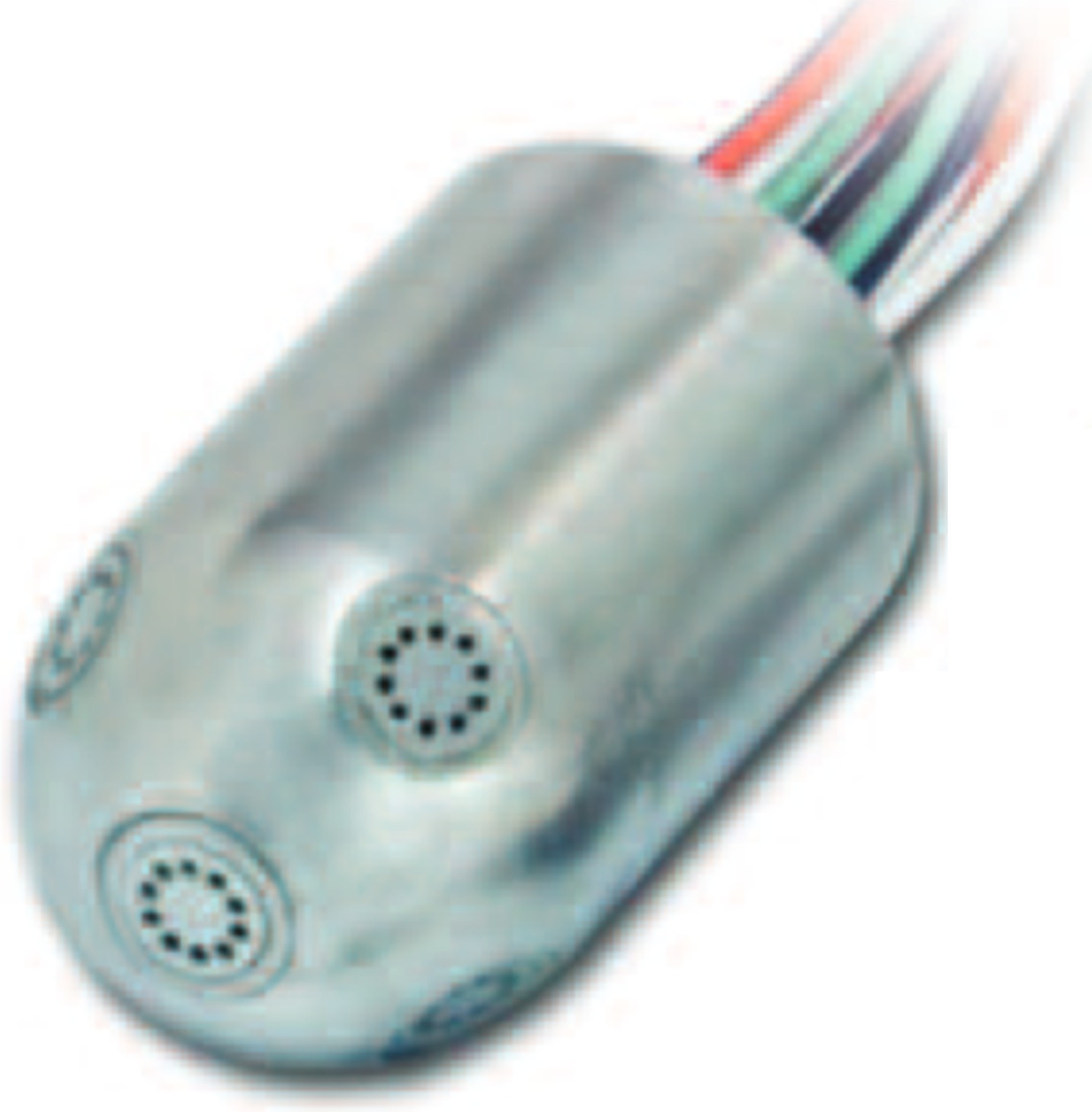
Unsteady flow measurements are relatively commonplace, including velocimetry techniques such as hot-wires, Laser-Doppler-Anemometry and Particle-Imaging-Velocimetry. However, the quantification of aerodynamic loss requires the resolution of stagnation pressure as well as velocity. This requirement can be achieved by the use of fast-response pneumatic probes. For example, Figure 1 shows a 6-sensor probe from Kulite Inc, which can achieve a frequency response up to 200–380 kHz (Ned et al., 2013). However, the diameter of this probe is over 6 mm, which severely limits the spatial measurement accuracy; the typical width of compressor or turbine wakes in experimental rigs is of the order 2 mm (Grimshaw and Taylor (2016)). Other probe examples include the 4 mm diameter, 4-hole probe described by Chasoglou et al. (2018).
Smaller unsteady probes have been constructed with a reduced number of sensors, such as the single-sensor Fast-Response-Aerodynamic-Probes (FRAP) studied by a number of authors, e.g. Lenherr et al. (2011). These devices cannot measure instantaneous flow angles but multiple traverses can be used to reconstruct a steady or ensemble-averaged flow field, a technique demonstrated by Pfau et al. (2002).
The advent of Micro-Electrical-Mechanical-Systems (MEMS) has the potential to offer smaller sensors and reduce the size of unsteady probes. Rediniotis and Johansen (1998) examined a 5-hole MEMS probe with a diameter of approximately 1 mm, shown in cross-section in Figure 2. This probe includes a semi-spherical cap that is placed over a silicon chip with pressure sensors and was capable of a maximum frequency response of around 400 Hz. One of the major difficulties in constructing this probe was the fitting of the cap on top of the chip.

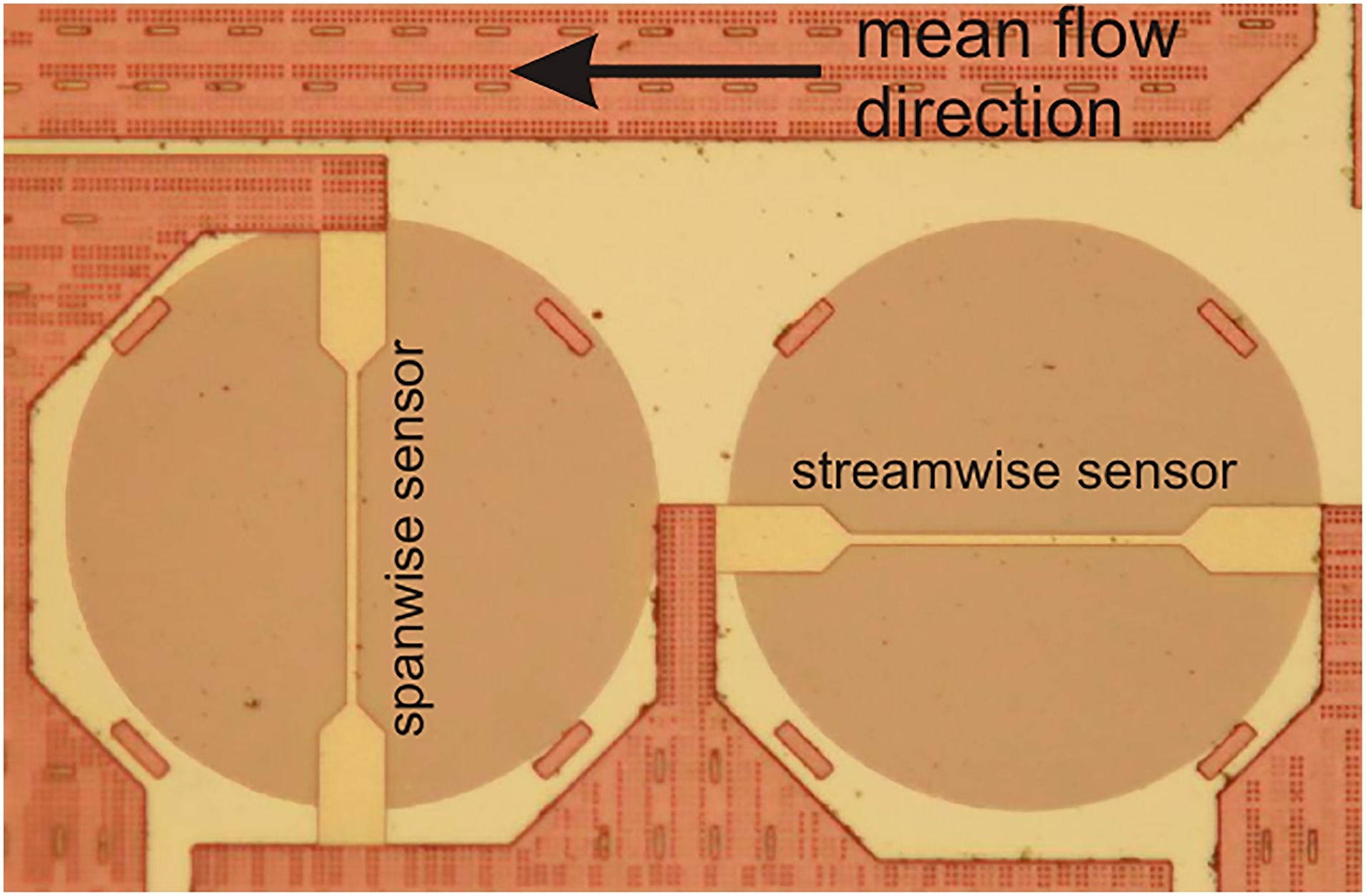
This paper considers an alternative approach to aerodynamic measurements that exploits MEMS directional shear stress sensors. An example is shown in Figure 3 (Evans et al., 2012) where two hot-film elements have been orientated at 90 degrees to each other. The directional sensitivity of this set-up is limited to around ±45° because the hot-films cannot distinguish between forward and reversed flow (though an additional sensor could extend the range to ±90°). Due to the low thermal mass and low conduction losses to the mounting membrane, this type of sensor can be designed to have a frequency response of up to 1 MHz (e.g. Haneef et al., 2007).
Figure 3.
Directional Shear Stress Sensor tested by Evans et al. (2012); two hot-film elements mounted on thin membranes.
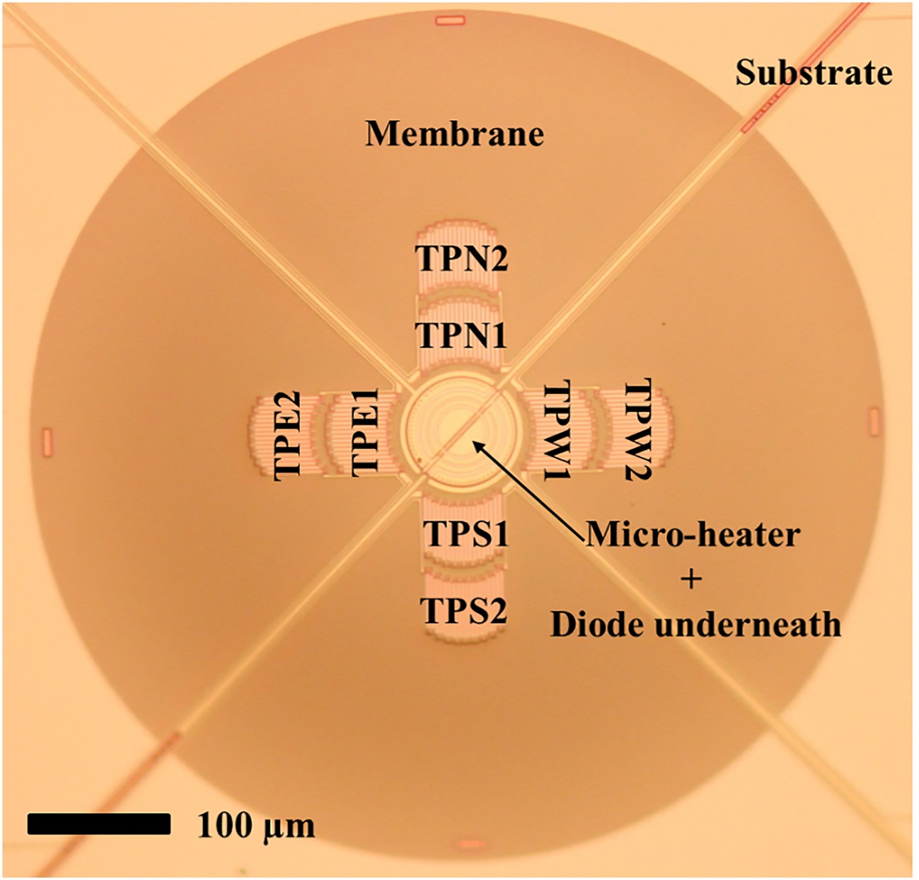
Another example of a directional sensor is shown in Figure 4, from De Luca et al. (2015b). Power is provided to a micro-heater at the centre of the membrane. The temperature distribution across the membrane surface is asymmetric due to the local shear force and direction, which can be measured by comparing the voltages across the thermopiles incorporated into the membrane. These sensors have the advantage of sensing flow angles across a full 360 degree range but have lower frequency response than the designs in Figure 3.
Figure 4.
Directional MEMS shear stress sensor incorporating microheater and thermopiles (TP) on a thin membrane; De Luca et al. (2015b).
The probe concept studied in this paper uses directional shear stress sensors and pressure sensors, all of which could be incorporated onto a single MEMS chip (e.g. Mansoor et al., 2016). The design avoids the need for a cap over the sensor chip and has the potential to achieve high temporal and spatial resolution in a relatively simple package. The following sections of the paper describe:
Principles of operation
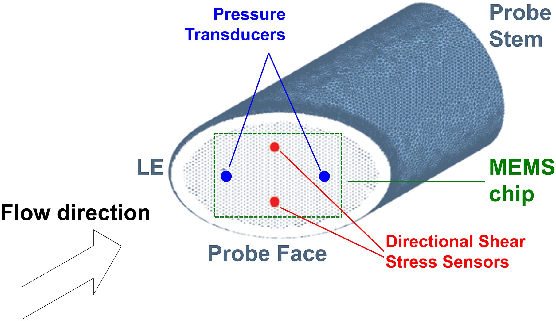
Figure 5 shows a schematic of the novel probe concept. The design exploits recent progress in MEMS technology, in particular the development of multi-sensor chips (e.g. Mansoor et al., 2014). The head of the probe consists of a cylinder with an angled face, upon which a single MEMS chip containing several sensors is mounted. The leading edge (LE) of the angled face is radiused to minimise flow separation at incidence. Thanks to the single chip, this relatively simple set-up has the potential to be miniaturized to achieve a stem diameter of around 1 mm.
Flow angle sensitivity
Two shear stress sensors are located towards the top and bottom of the MEMS chip (Figure 5). Rather than considering the absolute levels of shear stress, these sensors are used to measure the local direction of the near-surface flow. This local direction depends on the freestream flow angles, which determines the position of the stagnation point on the probe face and the streamline pattern over the face. In the absence of separations, this flow pattern is determined by the inviscid stagnation flow and therefore has minimal Reynolds number dependency.
The sensitivity of the probe to yaw angle is illustrated schematically in Figure 6. The yaw angle is defined in the vertical plane relative to the probe. For zero incidence the stagnation point is close to the leading edge of the probe, and the two sensors give symmetric angles. An increase in yaw angle
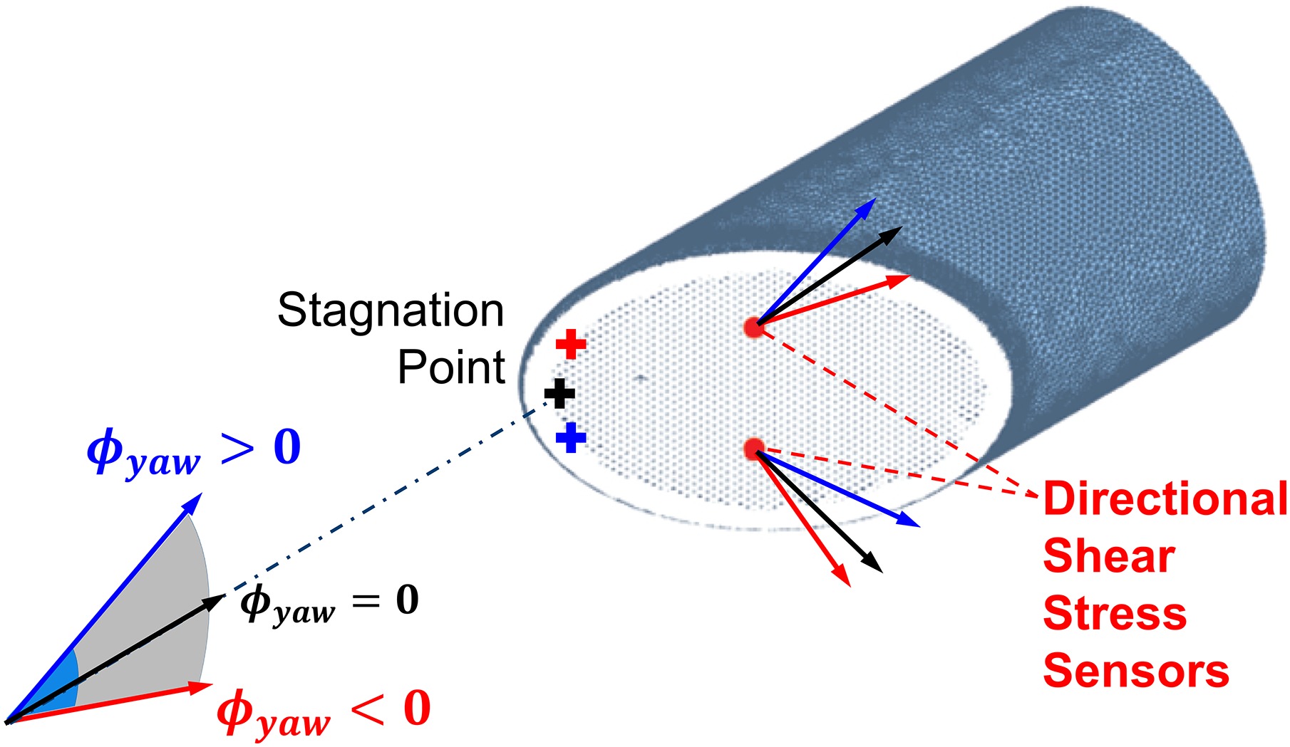
Figure 8.
Computed surface streamlines and stagnation point (yellow dot) on the face of a probe with 45° face at different flow angles; view from upstream.

Figure 7 illustrates the response of the probe to variations in pitch angle, which is here defined in the horizontal plane relative to the probe. A positive pitch angle causes the stagnation point to move further aft on the probe face (Figure 8), increasing the difference between the angles measured by the two sensors. In contrast, a negative pitch angle causes the stagnation point to move towards the leading edge, causing the measured flow angles to become more parallel. Thus, the difference between the sensor angles is sensitive to the pitch angle.
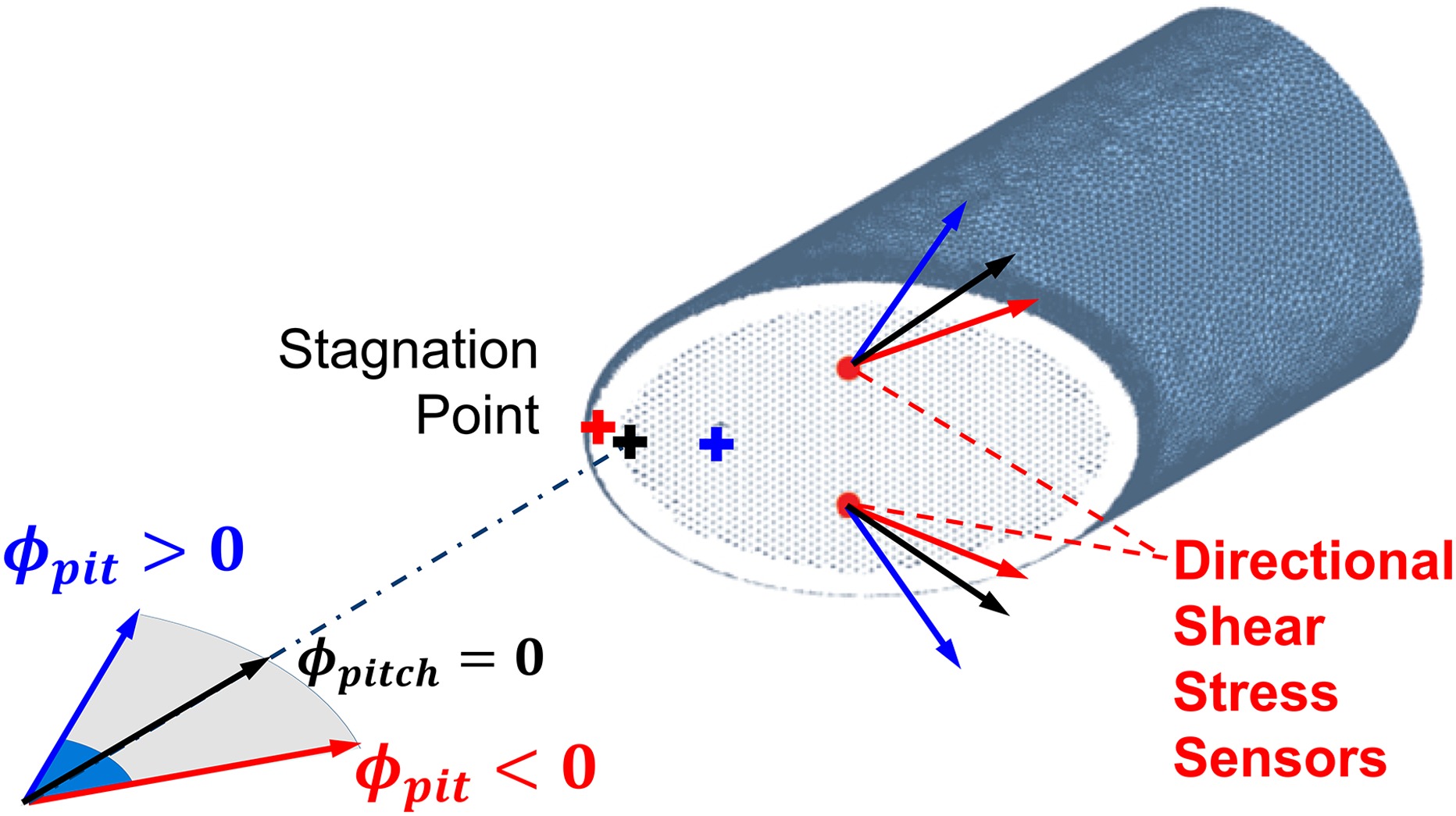
At extreme negative pitch angles, the stagnation point moves onto the side face of the probe (to the left of the leading edge in Figure 7) and produces a leading edge separation. This behaviour limits the negative pitch range of the probe but can in part be mitigated by applying a radius to the leading edge.
Pressure and temperature
Stagnation and dynamic pressure can be measured via the two pressure transducers flush-mounted on the MEMS chip: the foremost one reading a value closer to stagnation pressure and the rear one closer to static (Figure 5). Javed et al. (2019) reviews the principles and application of such MEMS pressure sensors, which are typically one to two orders of magnitude smaller than traditional transducers. Like all transducers, these sensors are sensitive to temperature. Compensation would be provided by on-chip temperature measurements as described by the review of Mansoor et al., 2015. Thus, when suitably-calibrated, the final probe should also be capable of measuring stagnation and static temperature and pressure.
Frequency response
Though not addressed directly in this paper, it is useful to consider the likely frequency response of the concept probe. The MEMS sensors shown in Figure 3 can be designed to have a frequency response significantly greater than 100 kHz, and as high as 1 MHz (Haneef et al., 2007). Overall, the frequency response of the probe is more likely to be limited by the fluidic time constant governing the response of the surface streamlines to changes in the freestream flow.
A simple estimate of the fluidic time constant t for an aerodynamic probe can be made by considering a reduced frequency based on the probe diameter and flow velocity:
A reduced frequency below ∼0.3 is typically required for quasi-steady flow. Thus the likely maximum frequency response of the probe may be estimated as:
Equation 2 demonstrates that miniaturisation is necessary to achieve a high frequency fluidic response. For example, a 1 mm diameter probe with a flow velocity of 100 m/s will have a fluidic frequency response of around 30 kHz, broadly similar to a hot-wire. In contrast the 6 mm probe in Figure 1 would achieve only around 5 kHz at the same conditions. Thus, the miniaturisation promised by the novel probe described in this paper has the potential to offer a step-change in temporal accuracy.
Computational design study
A design study was performed using Computational Fluid Dynamics (CFD) to understand how the probe geometry and sensor layout should be designed to maximise sensitivity and useable range. Particular attention is paid to the angle sensitivity since the mechanism exploited by the probe is very unlike any existing device.
For this initial study the inlet Mach number and the Reynolds number were held constant at 0.25 and 3010 respectively. This Reynolds number corresponds to a probe diameter of 2 mm at standard atmospheric pressure and temperature. A systematic set of freestream pitch and yaw angles were calculated for each probe geometry. For simplicity all virtual sensor outputs were obtained for single node points.
Computational methods
The CFD domain is shown in Figure 9. A defined velocity vector is specified at the pressure-far-field inlet, which is hemispherical with a radius of 8 probe diameters. The cylindrical exit plane is specified as a pressure outlet and is located five probe diameters downstream of the leading edge. Unstructured meshes were generated using ICEM. Prismatic surface layers were used on the probe face, with a y+ value of approximately unity on the surface, an expansion ratio of 1.15 and 20 layers. The resulting meshes have around 1.5 million cells and further refinements did not change the solutions (Morris, 2017). Reynolds-Averaged-Navier-Stokes (RANS) calculations were performed with Fluent v16.0 using a coupled, pressure-based numerical approach.
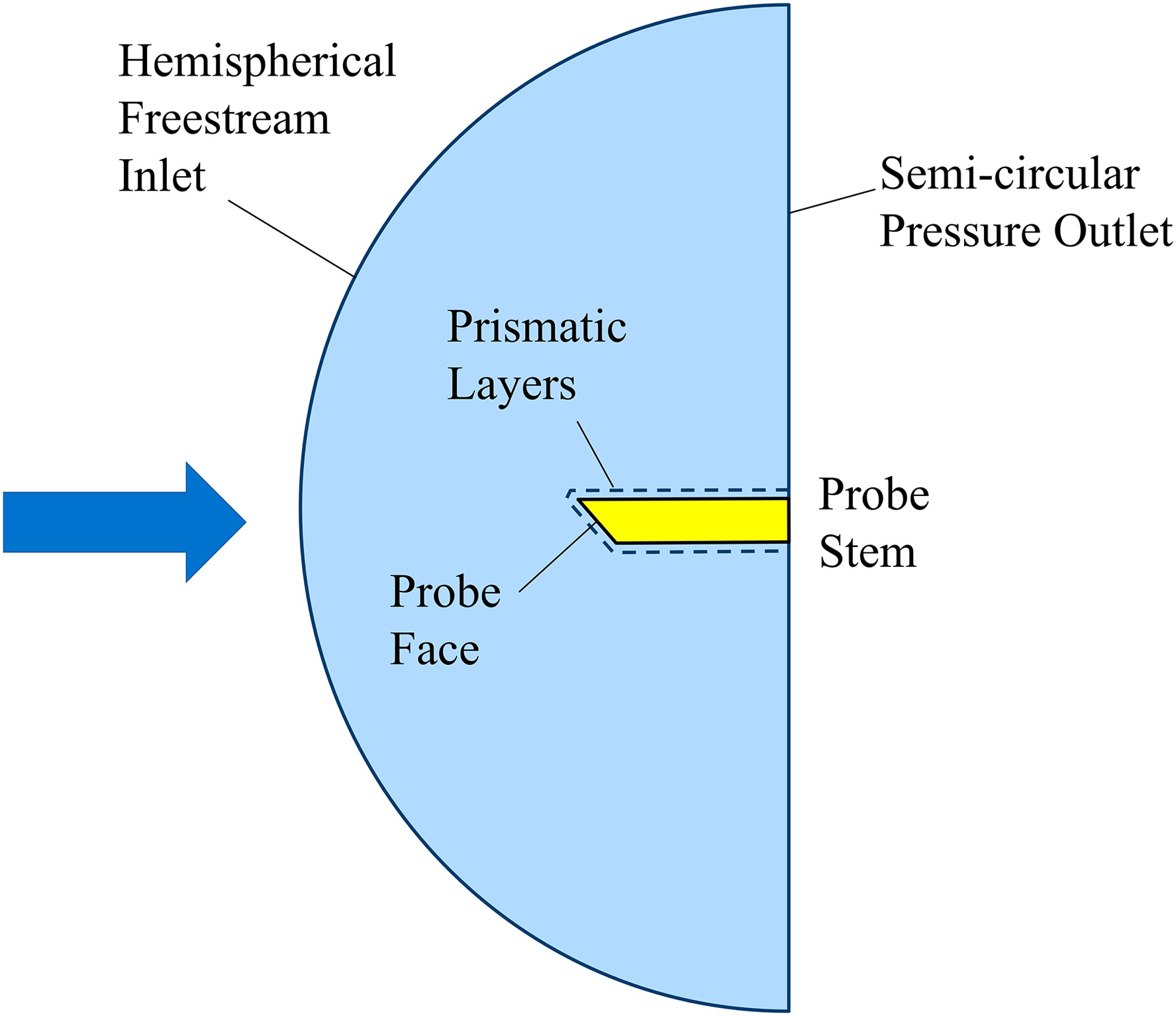
There will be considerable laminar flow on the probe head at this Reynolds number (3010) which is challenging to model. Laminar calculations typically suffer from convergence problems, while the available transition models have not been sufficiently validated of for this type of flow. Therefore, fully turbulent flow was assumed using the kω-SST model. This approximation is not expected to significantly alter the surface streamline directions or pressure field on the probe head, which are largely determined by inviscid mechanisms.
Baseline probe: sensor location
The “baseline” probe geometry shown in Figure 5 has a face angle of 45° and a small leading-edge radius equal to 2% of the probe diameter. The choice of location for the directional shear stress sensors requires a balance of multiple considerations:
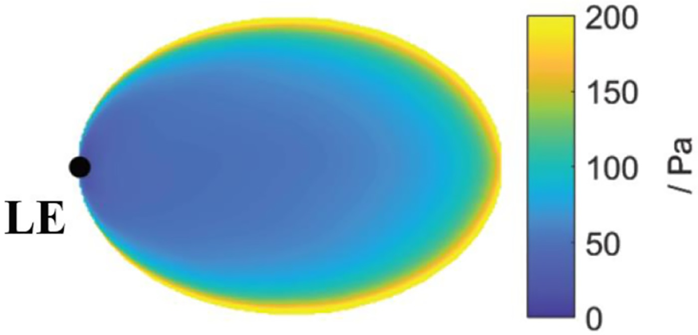
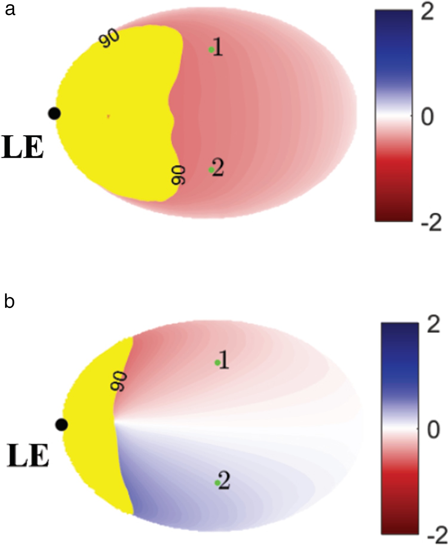
The magnitude of the local shear stress. Placing the sensors in regions of low shear will cause signal-to-noise issues and should therefore be avoided. The predicted shear stress magnitude at zero pitch and yaw angle is shown in Figure 10. Sensor locations in the low shear stress regions close to the leading edge are undesirable.
High sensitivity of the local flow direction to the freestream flow angles; since high sensitivity will improve the accuracy of the probe.
Flow direction variations remain within a 90° range across the calibration map. This requirement enables the use of the highest-frequency response sensors shown in Figure 3.
A valid calibration map can be generated over a large range of incidence angles, i.e. it is possible to calculate a unique set of freestream angles given the local flow angles at the sensors. Pneumatic five-hole-probes typically have valid calibration maps within a range of ±30° in yaw and pitch.
The shear stress angle
Figure 11.
Sensor Angle Variation: (a) yaw variation at zero pitch angle; (b) pitch variation at zero yaw angle. The calibration coefficients from Equations 3 and 4 are included.
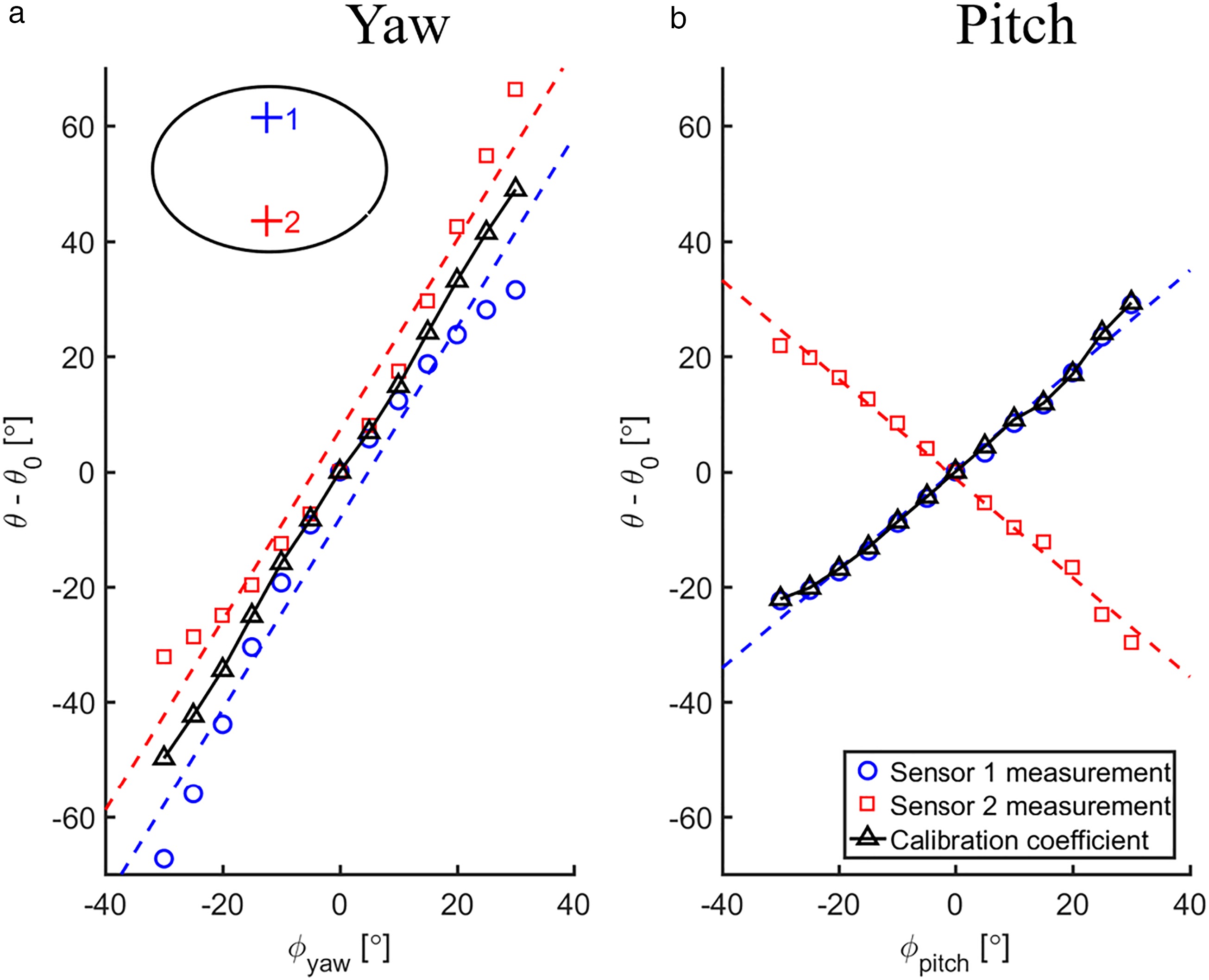
Two simple calibration coefficients are defined for the probe. For yaw variations the two sensor angles tend to move in unison and therefore a simple mean angle is used to define a Yaw Coefficient:
where 1 and 2 indicate the two sensors. For pitch variations, the two sensor angles tend to move in opposing directions and the difference is used to define a Pitch Coefficient:
These coefficients have been added to Figure 11 and can be seen to give almost linear response with freestream angles.
Plots similar to Figure 11 can be generated for alternative sensor locations over the blade. To indicate the sensitivity across the probe face, a least-squares linear fit is performed for each point:
where a and b are constants; the slope a is a measure of the sensitivity:
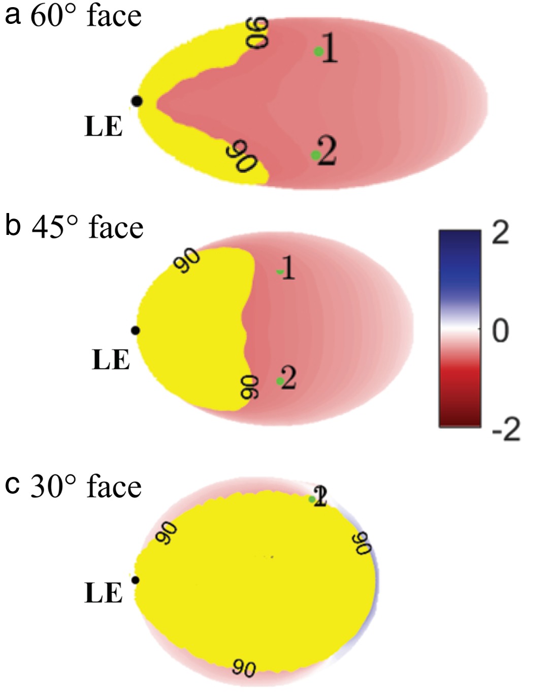
Figure 12a and b present maps of the sensitivity a for yaw and pitch angles respectively. In line with requirement (3) above, regions where the sensor angles varied by more than 90° need to be avoided and have been coloured yellow in these plots. In general, these regions are close to the leading edge where small movements in the stagnation point can lead to large changes in the flow direction. Over the remainder of the maps, the sensitivity to yaw (Figure 12a) is relatively uniform, while pitch sensitivity can be maximised by moving the sensors outboard towards the edge of the probe face (Figure 12b).
Figure 12.
Maps of sensitivity a in Equation 5: (a) yaw sensitivity at zero pitch angle; (b) pitch sensitivity at zero yaw angle. Yellow regions indicate a local flow angle range in excess of 90°.
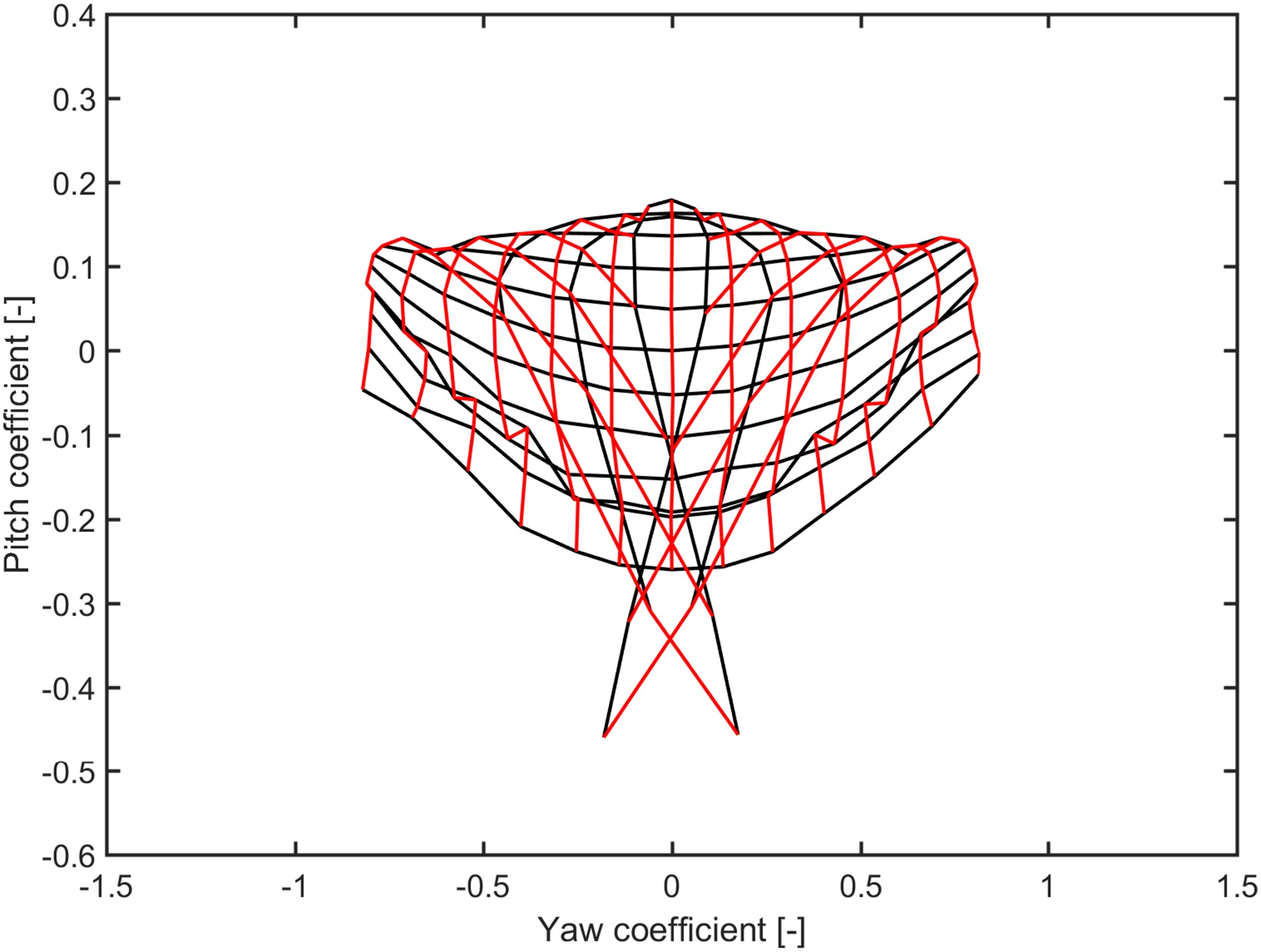
To examine the combined variation of pitch and yaw angles a virtual calibration map is presented in Figure 13 for the baseline probe with sensor locations 1 and 2 (Figure 12). The coefficients are presented in radians. The map is presented as a “spider” map, with increments of 5° in pitch and yaw angle. Black lines of constant pitch angle and red lines of constant yaw angle are indicated on the plot, and the zero-incidence point is indicated by the black dot in the centre of the map. The sensitivity of the probe is indicated by the rate of change in coefficients as the flow angles vary. Over most of the range the probe gives a valid map and has a useable range of at least ±20° in yaw and −20° to +30° in pitch. Outside this range, some folding of the map is evident for negative pitch angles (<−20°) and extreme yaw angles, as indicated in the inset plot to the top left of the plot. In these folded regions there is no unique set of flow angles for a given yaw and pitch coefficient and the calibration cannot be inverted. The CFD solutions show that this behaviour corresponds with the movement of the stagnation point to the outside face of the probe, causing separation over the leading edge. In addition to the folding at the extremes of the map, there is an undesirable “pinching” of the −15° and −20° pitch lines at ±20° yaw, which will cause high errors in this region (see Figure 21). It is noted that a more complicated approach to the calibration (e.g. using machine learning algorithms) would likely extend the useful range of the probe, but the simple coefficients in Equations 5 and 6 are sufficient for the current purpose of demonstrating the probe concept.
Figure 13.
Virtual calibration map for default sensor positions (1 and 2 in Figure 12); baseline probe.

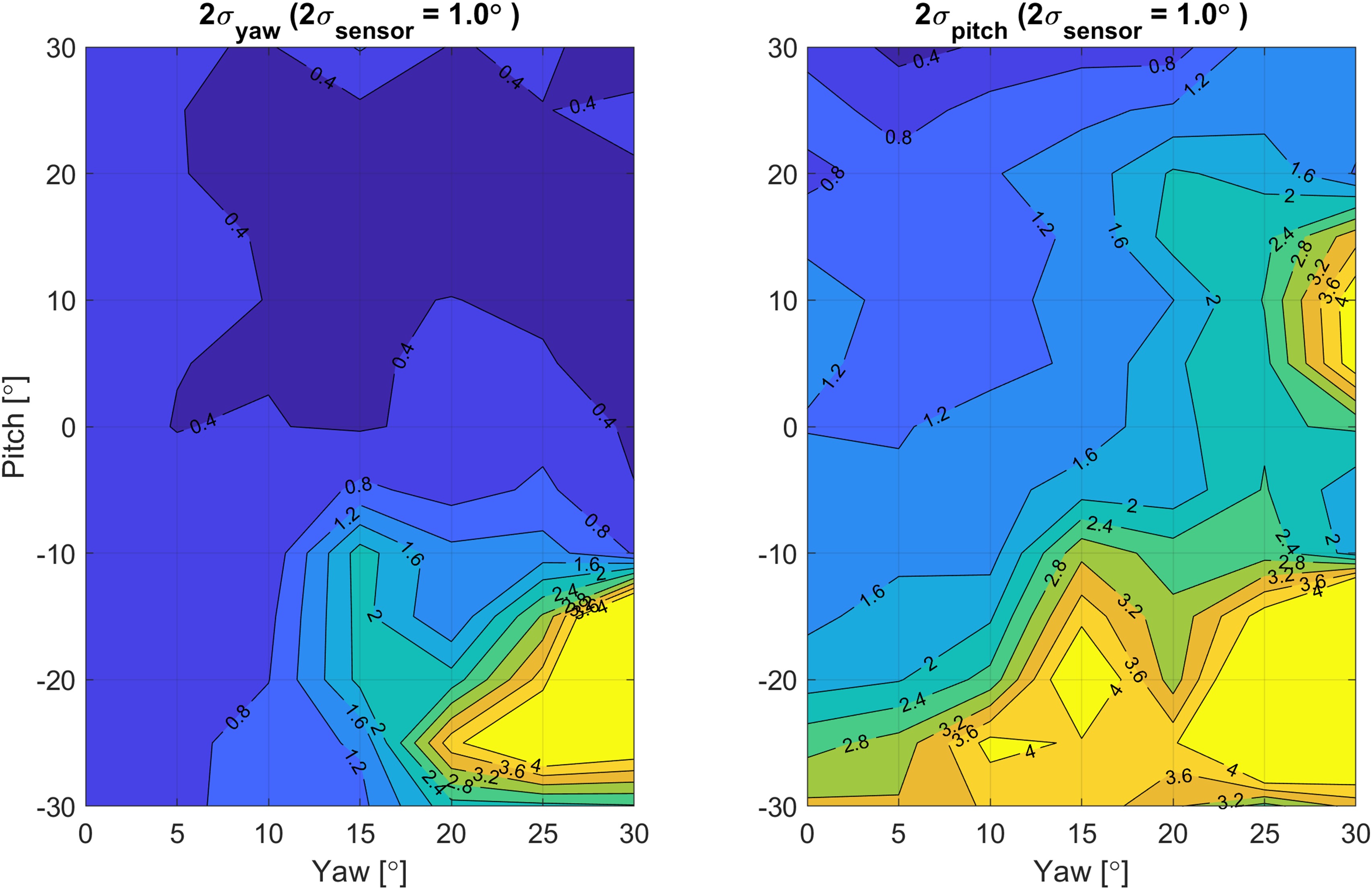
Figure 14 shows the impact of sensor location on the calibration map, by moving the sensors forwards, rearwards, inboard and outboard. The map from Figure 13 is reproduced in Figure 14c for reference. Only symmetric movements of the two sensors are considered.
Figure 14.
The impact of shear stress sensor locations on the virtual calibration map; baseline probe.
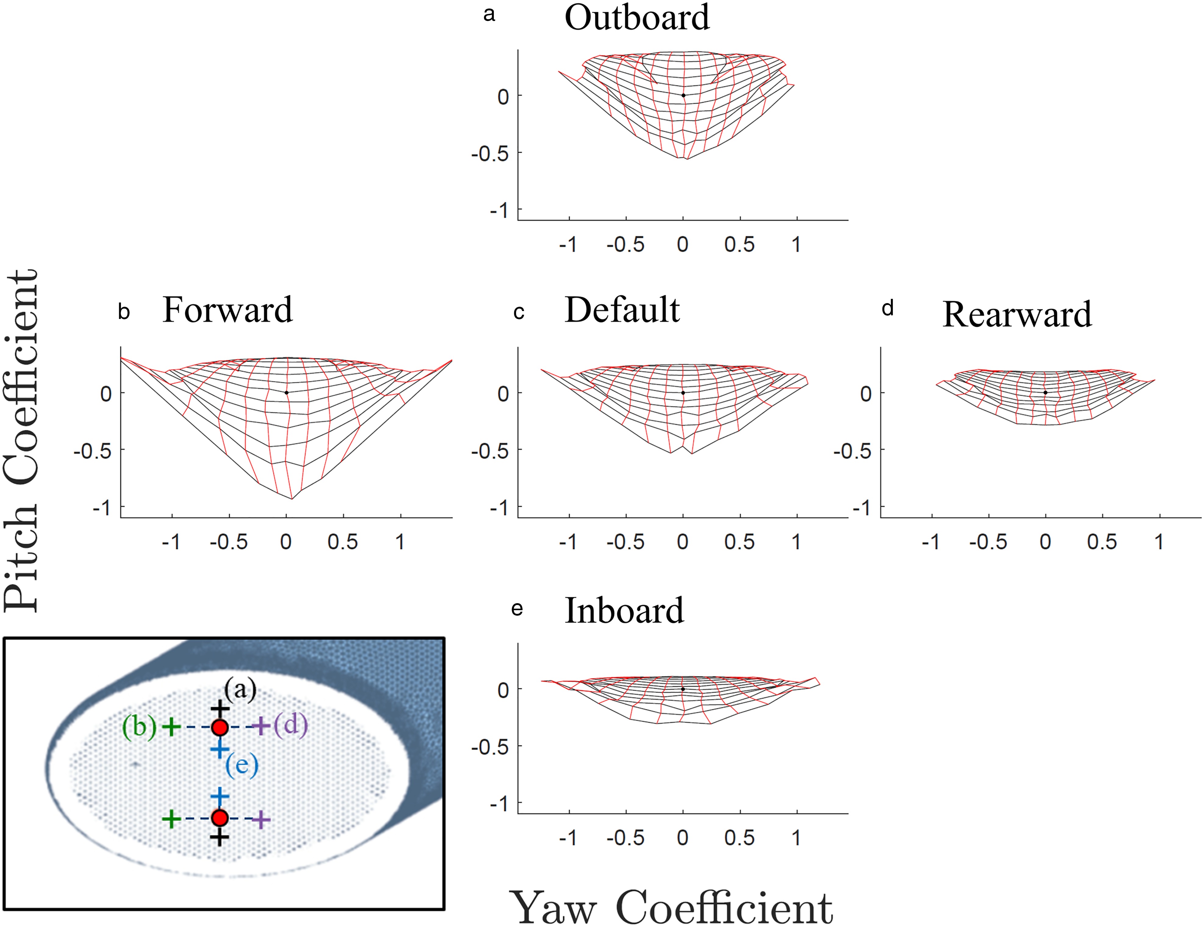
Moving the sensors forwards towards the leading-edge results in larger angle variation due to their proximity to the stagnation point. As a result, the sensitivity increases causing the calibration map to spread out (Figure 14b vs. c). However, these sensor locations are also close to the separation regions at extreme negative pitch, causing a larger region of map folding and a reduction in the useable range. In a similar manner, moving the sensors rearward (Figure 14d vs. c) reduces both the sensitivity and the map folding.
Moving the sensors outward on the probe face (Figure 14a vs. c) increases the pitch sensitivity, in line with the increased sensitivity towards the top and bottom of the probe face in Figure 12. However, these probe locations are also more susceptible to map folding at extreme negative pitch angles. Similarly moving the sensors inboard (Figure 14e vs. c) reduces the pitch sensitivity and reduces the map folding.
Clearly, the choice of sensor location requires a balance between the sensitivity and operating range. The calibration maps in Figure 14 also highlight the issues of this probe at extreme negative pitch angles. It is shown below that increasing the leading-edge radius can mitigate this problem and extend the operational range.
Probe face angle
Alternative probes with face angles of 60° and 30° were considered to observe the impact on the sensitivity. Figure 15 presents the yaw sensitivity for each design; Figure 15b reproduces the result from Figure 12a for ease of comparison. Again, the regions with flow angle variations greater than the range of the sensors (90°) have been indicated by the yellow regions. The sharper leading edge of the 60° probe tends to give less movement of the stagnation point. This effect is evident in Figure 15a which shows a larger usable area of the probe compared to Figure 15b. For the 30° probe, the probe face is more normal to the incoming flow direction and the stagnation point moves over a wide area of the probe. As a result, most of the surface observes wide swings in angle and therefore this design is not compatible with the sensors shown in Figure 3.
Figure 15.
Yaw Sensitivity (a
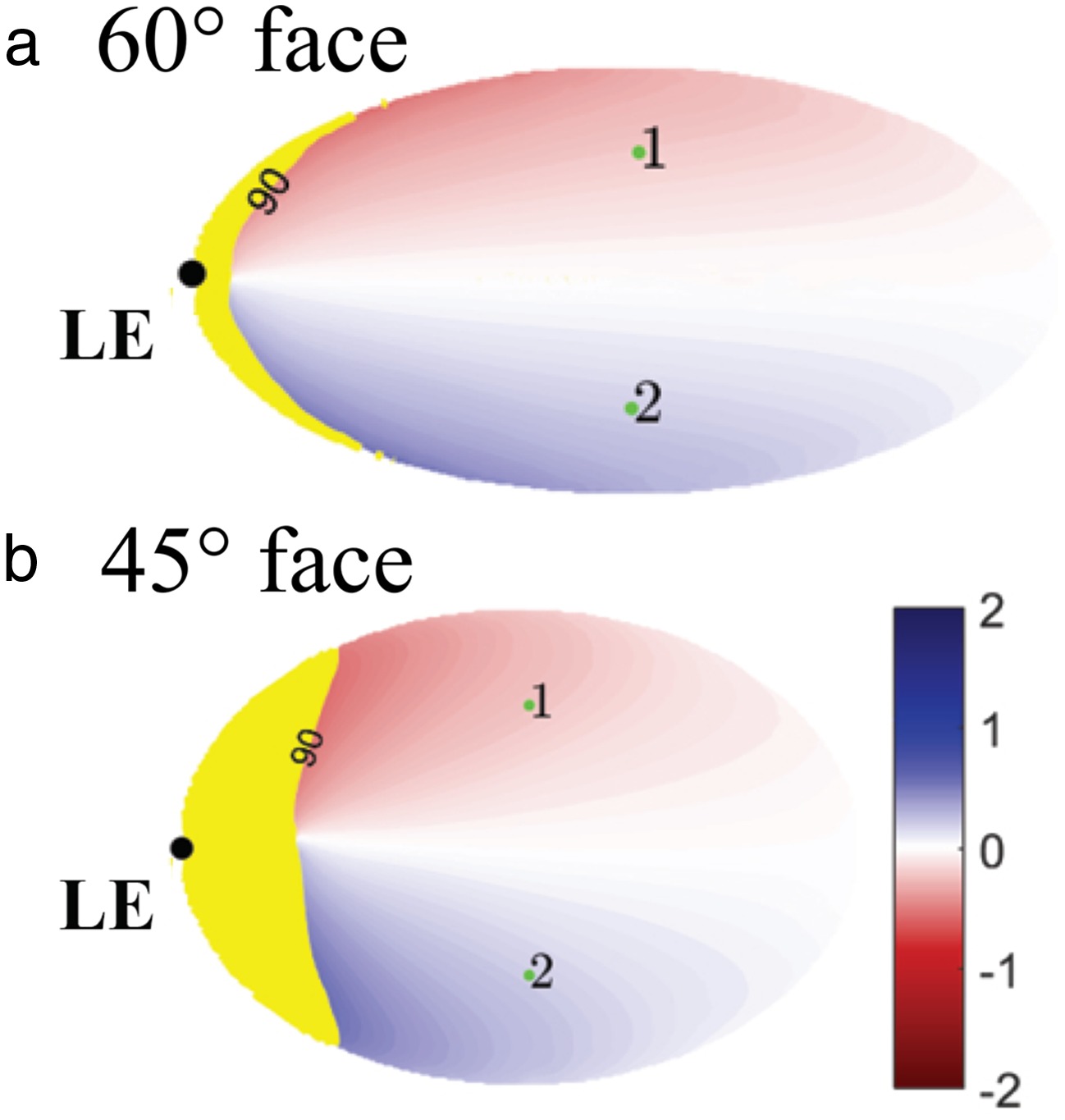
The increased face angle of the 60° probe tends to cause the flow to align more closely with the probe axis. As a result, the pitch sensitivity for the 60° probe (Figure 16a) is slightly lower than for the 45° probe (Figure 16b). Using the sensor locations 1 and 2 in Figures 16a and 17 shows the calibration map for the 60° probe. Compared to the 45° probe (Figure 13), it can be seen that the pitch sensitivity is reduced and the map folding at negative pitch angles is more pronounced, which is the result of a more severe separation from the sharper leading edge. Based on this comparison, the 45° probe gives a wider operating range and better sensitivity and was therefore selected for further investigation.
Figure 16.
Pitch Sensitivity (a
Leading edge radius
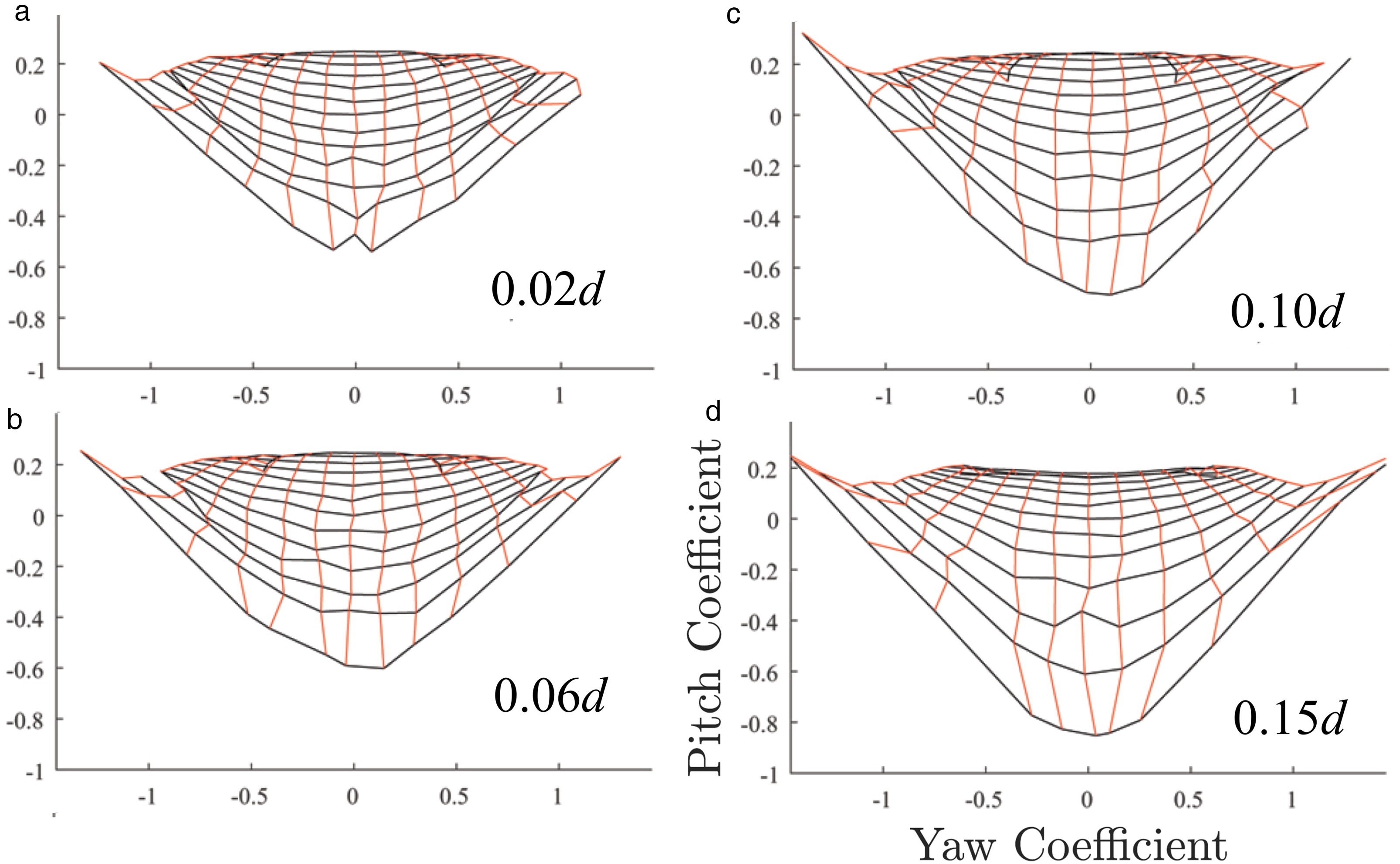
One limitation of the baseline 45° probe is the behaviour at large negative pitch angles, where leading edge separation affects the results. To mitigate this problem, the radius of the leading edge was progressively increased, as shown in Figure 18. Calibration maps for the four edge radii are presented in Figure 19. A larger radius allows the stagnation point to move smoothly around the leading edge and minimises separations. It can be seen that the largest radius (Figure 19d) reduces the folding in the map at extreme negative pitch angles, extending the usable range to ±30° in yaw and −20° to +30° in pitch for the largest radius (15% of diameter). This “final” geometry was therefore selected for the experimental demonstrator. It is noted that further increases in radius are hindered by the need to maintain a sufficient flat surface to mount the sensor chip (Figure 5).
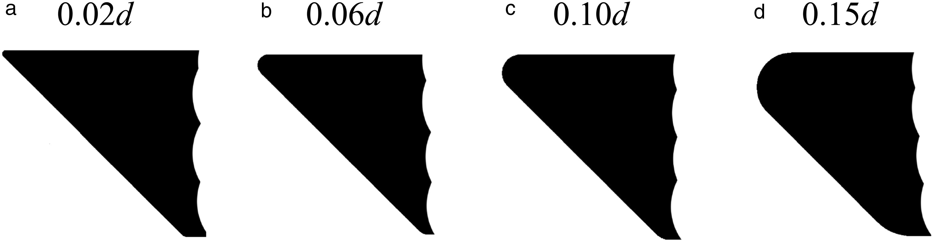
Figure 19.
Calibration maps for varying leading edge radius; 45° probe, sensor locations 1 and 2 (Figure 12); range of ±30° in pitch and yaw.
Stagnation and dynamic pressure
The location of the two pressure transducers in Figure 5 is relatively straightforward. Figure 20a shows the variation in static pressure coefficient over the face of the final probe (
Figure 20.
Predicted stagnation (C p , 0 C p , d y n α β

where
The stagnation pressure coefficient is taken as:
where
Figure 20b and c present contour maps of the two coefficients over a range of ±30° in yaw and pitch. The stagnation pressure coefficient (Figure 20b) is close to zero at positive pitch angles, when the measured pressure is close to stagnation. The dynamic pressure coefficient (Figure 20c) reaches a minimum at approximately zero incidence, where the pressure difference between the two transducers is maximised. This trend is also visible in Figure 20d and e, which present the two coefficients for isolated changes in yaw and pitch respectively. At −30° pitch and extreme yaw angles the coefficients invert (Figure 20b and c) as the pressure on sensor
Accuracy estimation
An accuracy estimate of the probe can be obtained by making assumptions about the likely accuracy of the individual sensors. Here a sensor angle sensitivity of
Experimental demonstration
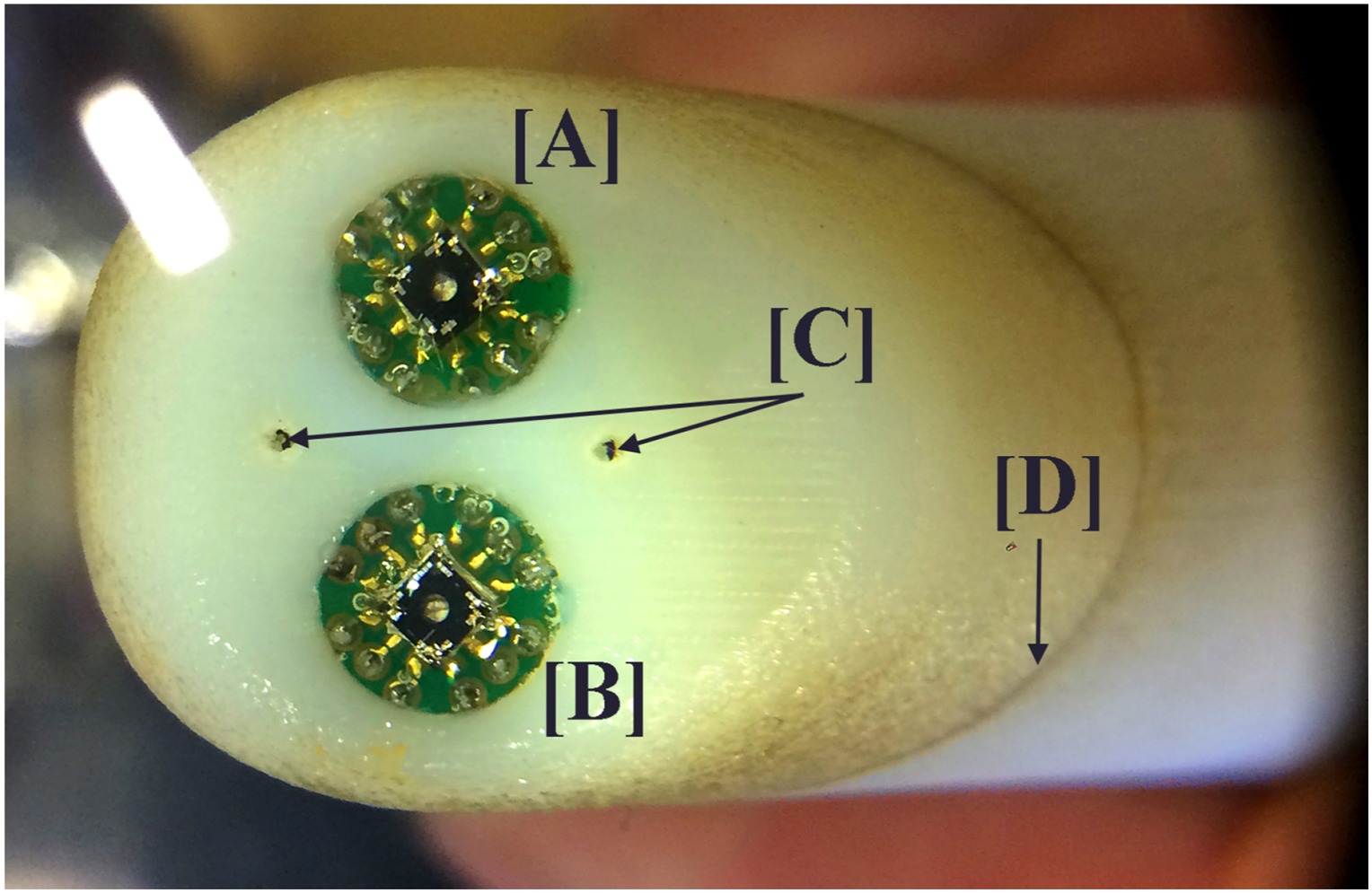
In order to provide a first demonstration of the probe concept, a steady calibration was performed using a large-scale model. The test probe was constructed using 3D printing and has a diameter of 16 mm, which allowed the use of existing MEMS sensors without the need to fabricate dedicated chips. The large scale also facilitated the mounting of these sensors into the probe using the standard packaging techniques that were available. Figure 22 and Figure 23 show the CAD model and a photo of the probe head.
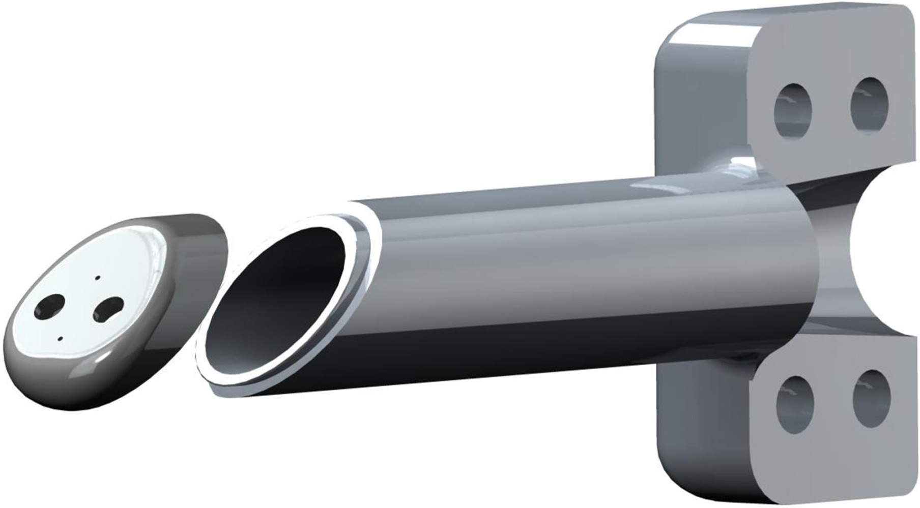
Figure 23.
Experimental Probe Head: MEMS shear stress sensors (a, b – see Figure 4); static pressure tappings (c); probe stem (d).
Measurements
Due to availability, shear stress sensors of the design shown in Figure 4 were used in the experiment. The relatively low frequency response of these sensors is inconsequential for this steady demonstration.
A direct replication of the CFD yaw and pitch coefficients would require that each sensor is first independently calibrated for angle and shear stress before the probe can be calibrated. By assuming each sensor has similar thermoelectric properties, the Appendix shows that a good approximation to the shear stress angle can be obtained directly from the sensor output voltage, thereby eliminating the need for a separate shear stress calibration (Equation 10). In practice for a real probe, any minor errors caused by making this assumption would be eliminated by directly calibrating the “voltage angle” to the flow angle in a known flow, in much the same way as a current pneumatic five-hole probe.
where
Measurements were performed in a calibration wind tunnel in the Whittle Laboratory, Cambridge at a velocity of 57 m/s, corresponding to a probe Reynolds number of around 66,000. Pressures are measured using static pressure tappings in the head of the probe, [C] in Figure 23, and were recorded using a Scannivalve DSA 3217 with a 10” H20 range, with an uncertainty of around 0.06% of dynamic head. Total and static pressure in the calibration jet were measured with reference probes. Yaw and pitch angles of ±30° were tested in increments of 10°. A Keithly 2401 DAQ was used to measure sensor output voltages.
Angle sensitivity
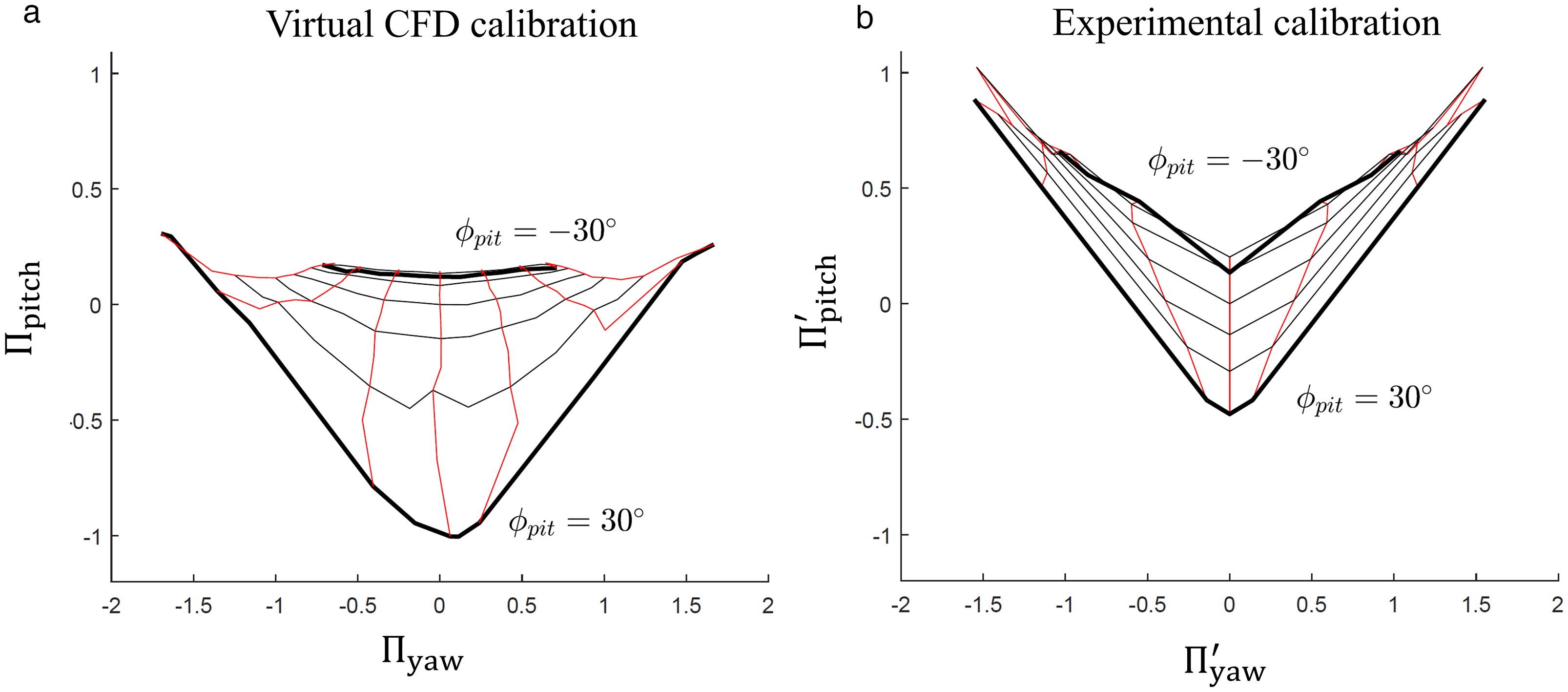
Upon installation it was found that one of the MEMS sensors had been damaged and generated high levels of noise. A calibration map was therefore reconstructed by taking data from the single working sensor and mirroring it, effectively assuming perfect yaw symmetry of the set-up. The resultant calibration map is compared to the predicted map in Figure 24. In general, the probe behaves in a similar way to the predictions. The useable range of the experimental map matches the computation and is valid for approximately ±30° in yaw and −20° to +30° in pitch. The shape of the two maps is also generally similar, but the experimental pitch coefficient is generally higher than the computed value. This effect is believed to indicate limitations in the quasi-angle assumption in Equation 10. In any case, the final probe will use high-frequency response sensors as in Figure 3, which have different characteristics.
Stagnation and static pressure
The measured stagnation and dynamic pressure coefficients

Conclusions
A successful concept demonstration of a novel MEMS-based aerodynamic probe has been performed. The probe uses directional shear stress sensors on an angled face to determine the flow direction. The current configuration is capable of measuring flow angles in a range of ±30° in yaw and −20°/+30° in pitch. By incorporating different sensors onto the MEMS chip, the probe will be capable of measuring stagnation pressure, dynamic pressure and temperature. The design can be miniaturised to around 1 mm diameter and should offer a step-change improvement in temporal and spatial resolution compared to existing unsteady probes.
A computational study of the probe and sensor layout has given some insight into the design trade-offs. Particular attention has been paid to the unusual method of flow angle measurement:
A 45° face angle gives a good compromise between sensitivity and operational range. A 30° face angle improves sensitivity but the swings in local angle are beyond the sensing range of the shear stress sensors; a 60° face encourages leading edge separation at negative pitch angles and reduces the operational range.
Radiusing of the probe leading edge can extend the operating range of the probe by supressing separation at negative pitch angles.
Moving the shear stress sensors forward on the probe face increases sensitivity but decreases the operational range.
Moving the shear stress sensors outboard on the probe face increases the sensitivity to pitch angle but decreases the operational range.
The pressure coefficients invert at extreme negative pitch angles where the angle map folds, thus warning of out-of-range operation.
Future work will be required to further optimise the configuration, improve the calibration method, miniaturise the device, assess measurement accuracy in more detail and characterise the frequency response of the probe.
Nomenclature
Pressure Coefficient, Equation 7
Stagnation Pressure Coefficient, Equation 8
Dynamic Pressure Coefficient, Equation 9
Probe Stem Diameter
Voltage
Frequency
Reduced Frequency
Freestream stagnation pressure
Freestream static pressure
Surface static pressure
Transducer pressures
Velocity
Fluidic time constant
Sensor shear stress angle
Voltage-based quasi-shear-angle, Equation 10
Pitch Coefficient (CFD), Equation 4
Yaw Coefficient (CFD), Equation 3
Experimental Pitch Coefficient, Equation 12
Experimental Yaw Coefficient, Equation 11
Shear Stress
Freestream Pitch Angle
Freestream Yaw Angle