Introduction

Considering the unsteady flow in an axial turbomachine, the frequency spectrum of the fluctuations is in the range of a few hertz up to several multiples of the blade passing frequency. For gaseous-flows in turbomachines, frequencies up to 50 kHz are, in most cases, of practical interest (Kupferschmied et al., 2000). The time and length scales of the flow structures vary up to six orders of magnitude, due to the diverse nature of the originating mechanism 1. Periodic fluctuations arise due to regular wake passing or other secondary and leakage flow features, or even shocks 10. On the other hand, stochastic fluctuations can be attributed to turbulence, to unsteady transition, separation of boundary layers, etc. In order to understand the loss mechanisms under these conditions, experimental work and computational tools must come together to evaluate the flow structures. A comprehensive review of measurement techniques for unsteady turbomachinery flows can be found in 2, 32.

Despite the advancements in numerical modelling and computational tools, turbulence models are mainly based on a series of assumptions or simplifications, which may be mathematically plausible but do not necessarily accord with the actual physics in a turbulent flow. Nevertheless, turbulence modelling is inherently connected to the design and development process in internal turbomachinery applications. In the past numerical tools were validated through experimental investigations in simplified test rig geometries, while lately the interest has shifted towards experimental data acquisition under realistic complex flow conditions 9, 25, 20.

In most studies the turbulence quantities are derived from hot-wire anemometry measurements. However, the hot-wire probes suffer from their inherent fragility and loss of sensitivity at high Mach numbers which makes them suitable for lightly loaded, low-speed turbomachines. To overcome this issue fast-response pressure probes equipped with embedded piezo-resistive pressure sensors have been developed for highly loaded and high-speed turbomachines. Heneka was probably the first one to attempt deriving turbulence quantities with a 4-hole wedge unsteady probe 12. This probe was used for turbulence measurements in both freejet and high speed compressor by Ruck et al. 29, 30. 11 developed a miniature 4-sensor Fast Response Aerodynamic Probe (FRAP-4S), which was used to derive turbulence parameters in a pipe flow. In another work, 17 measured time-resolved flow quantities using a 1-sensor FRAP, assuming isotropic conditions and incompressible flow. 25 presented a methodology to infer turbulence quantities, for incompressible flows, in all three spatial directions, using the standard FRAP-2S under virtual 4-sensor mode (V4S) 24. Similarly, yawing a 1-sensor unsteady probe in different positions in order to derive the turbulent parameters was also demonstrated 23.

In the context of this work, the term multi-sensor will refer to unsteady probes with more than two sensors. In early designs, unsteady probes had surface mounted sensors 16, 8. To avoid sensor damage due to particle impact the latter probes’ sensors were also coated. Furthermore in 8, the probe design had a pneumatic hole to measure the total pressure in a time-average manner, a design option based on space limitations. The predecessor of Budecks’ probe is the wedge type probe designed by 12. The probe developed by 11 represents the most compact unsteady probe of its kind. To achieve a probe tip diameter of 2.5 mm, the yaw sensitive sensors had to be shifted in respect to the centre hole, thus resulting in a slightly larger sensing area than desired. Nevertheless, this remarkable design was discontinued and never used for turbomachinery measurements. It is worth noting, that the majority of the probes incorporate absolute pressure transducers, which limits the operating range of the proposed designs. In 7, an unsteady yaw probe is presented. This design incorporates interesting features, like the rectangular sensing ports to enhance the frequency response of the sensors and an air-bleed design. This latter feature is used to supply air at the trailing edge of the probe to stabilize the probe-induced wake and reduce errors due to unsteady lift and dynamic stall present in the current probe due to its asymmetric cross-section profile of the probe.

Finally, in 34 an L-shaped 5-sensor unsteady probe is presented, which is using the commercially available Kulite multi-sensor tip. The 6.35 mm tip was inserted to a 8 mm stem part. As reported from the manufacturer, the frequency response is rather high, of the order of 100 kHz, but the resulting probe diameter and the relative large distance between the circumferential pressure taps impacts substantially the spatial resolution. Furthermore, it should be mentioned that the rather large L-shaped tip design makes measurement in actual test rigs more challenging, since usually access holes for probe measurements range from 6 to 12 mm.

The current article presents the development and application of a newly designed FRAP-4S enabling the simultaneously measurement of the unsteady 3-dimensionnal flow velocity vector in turbomachines. In the subsequent sections, the design, manufacturing approach and calibration of the FRAP-4S are presented in detail. Then the probe performance is compared against the traditional FRAP 2-sensor (FRAP-2S) and 5-Hole Probe (5 HP) for accuracy assessment. Finally, a detailed analysis of the turbulence intensity distribution at the rotor exit of an axial turbine are presented and discussed in detail.

FRAP-4S probe description

The design, manufacture and operation of the newly developed fast response aerodynamic probe is based on longstanding experience gained over the last two decades at the Laboratory for Energy Conversion (LEC) at ETH Zürich (Kupferschmied et al., 2000; 22, 21; Bosdas et al., 2016, 2017). In more detail, the FRAP-4S is based on the well-established standard FRAP-2S. The FRAP-4S uses similar packaging and bonding solutions, but it has four miniature piezo-restive sensors embedded into the probe tip, instead of two for the FRAP-2S. The sensors were positioned underneath the sensing taps where the sensor’s membrane is protected from particle impact with a metal shield. The overall dimensions of FRAP-4S are provided in Figure 1, along with the pressure tap notation and the sign convention in the probe frame of reference. The probe has perpendicular facing holes with a diameter of 0.35 mm, while the included angle between the taps in the yaw plane is equal to 42°. The pitch sensitive sensor is positioned in the spherical tip where the tap is placed at 45° in respect to the centre hole (Figure 1).

Figure 1.

FRAP-4S probe tip schematic, relevant dimensions (in mm) and port annotation; (b) Actual probe tip; (c) Schematic of the Wheatstone bridge configuration.

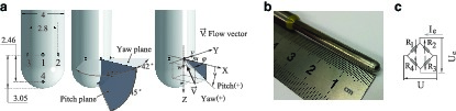
Compared to FRAP probes developed in the past at LEC the probe has a spherical tip head rather than the traditional filleted cylinder. The actual probe is shown in Figure 1. The probe tip diameter is 4 mm, which is connected to a 6.35 mm diameter stem located ten tip diameters from the tip (Figure 1). The overall length of the probe is 1 m. The main design challenges of the newly developed FRAP-4S were to accommodate the installation of four piezo-resistive pressure sensors within a miniature tip, while maintaining the required measurement bandwidth, sensitivity and robustness for applications in turbomachinery flows.

Piezo-resistive Sensor Static Calibration

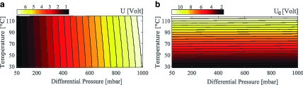
The FRAP-4S employs four miniature silicone piezo-resistive sensors, which incorporate the Wheatstone bridge configuration (Figure 1). Similar to the previously developed FRAP probes, the pressure-sensitive chips are operated under constant excitation current I_e. The induced excitation voltage U_e is primarily temperature dependent, while the resultant voltage output U is strongly dependent on the differential pressure induced athwart the sensor membrane.

For this study, the piezo-resistive sensors are calibrated over a differential pressure range and static temperature range of 50–1,000 mbar and 20–120°C respectively. The resulting U_e and U signal variation are shown indicatively in Figure 2 for one of the embedded sensors. Despite the increase in sensors’ packaging density, the quality of the static calibration results remains similar to the FRAP-2S 22. Moreover, the probe was subjected to a 40-hour thermal cycling test, in the aforementioned operating conditions. This long-term test showed no significant thermal drift for the sensors, while also maintaining excellent repeatability.

Figure 2.

Yaw sensor (sensor 1) calibration curves for pressure - U (a) and temperature - Ue signal (b).

Steady aerodynamic probe calibration

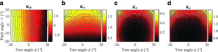
The FRAP-4S probe is calibrated in the free-jet facility of the LEC at ETH Zürich, more details regarding the operation of the facility can be found in (Kupferschmied et al., 2000). The calibration procedure is based on traditional methods described in (Kupferschmied et al., 2000; 15. A set of non-dimensional calibration coefficients is formulated from the probe’s pressure signal, total and static pressure of the flow. The coefficients are summarized in where K_φ and K_γ are the flow angle coefficients, K_t and K_s the total and static pressure coefficients respectively and p_m = (p₂ + p₃)/2.

(a)(b)

Kφ=p2−p3p1−pmKγ=p1−p4p1−pmKt=ptot−p1p1−pmKs=p1−pstatp1−pm

In the present work the probe was calibrated for Mach numbers of 0.3 and 0.5 at 30°C, (Re_D 25∙10³ and 43∙10³ respectively) conditions. The calibration maps are provided in Figure 3. In order to assess the probe’s aerodynamic performance, FRAP-4S is calibrated to a ±32° in yaw and pitch. The results have shown that the sensitivity of the probe pitch flow angle coefficient drops drastically for positive pitch angles, γ≥20° as the flow tends to separate on pressure port 4 for pitch incidence above 22°. The quality and the symmetricity of the obtained calibration curves proves the good accuracy during the manufacturing process.

Figure 3.

From left to right. FRAP-4S Aerodynamic coefficients for yaw, pitch angles, total and static pressure at M = 0.3.

Dynamic effects

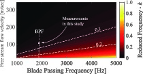
Fast response aerodynamic probes used for measurements in turbomachines are subjected to dynamic flow conditions. Strong velocity gradients and flow angle fluctuation are predominant in these type of flows and have shown to affect the accuracy of the measurement probe 13. Furthermore, in turbomachinery probe flow measurements the majority of the errors are proportional to the probe size and probe geometry (Kupferschmied et al., 2000). A non-dimensional parameter related to the degree of unsteadiness in the flow, is the reduced frequency k.

(2)

k=f⋅DC

In Equation 2, f represents the excitation frequency, i.e., the Blade Passing Frequency (BPF), D the probe tip diameter and C is the local free stream velocity. According to 13, the errors induced by dynamic flow phenomena are significantly reduced for cylindrical stem probes and for reduced frequencies below a critical value of k_crit = 0.1. Thus, the newly developed FRAP-4S has a diameter of 4 mm to reduce the impact on the unsteady measurement accuracy. Figure 4 illustrates the operating envelope of the probe, in terms of BPF and flow velocity, while also indicating the flow conditions in this study. The dashed lines indicate the critical value of k_crit = 0.1 and the k = 0.2 where lock-on of the Kármán vortex shedding occurs for the Reynolds number range of 25∙10³<Re_D<43∙10³, based on probe diameter.

Figure 4.

Reduced frequency versus BPF and free stream flow velocity.

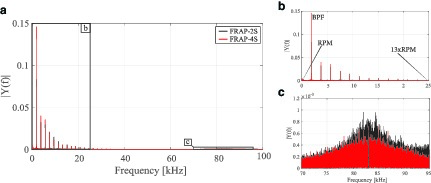
In order to obtain additional information regarding the dynamic effects on this new probe design, the pressure signal fluctuations were evaluated at different locations in the measurement plane at the exit of the rotor. In Figure 5 the frequency spectrum of the raw voltage signal U is provided for both FRAP-4S and FRAP-2S. These pressure signals refer to the center sensor, port 1, with both probes positioned at mid-span and in the middle of the stator pitch. There is a good overall agreement, while no frequency content related to amplitude amplification due to vortex shedding can be readily found, except from what is related to the rotational speed and the blade passing frequency modulation (Figure 5). Small peaks around the fundamental blade passing frequency are separated by a Δf = 45 Hz. Similar behaviour was observed by 26 and is attributed to the interaction of the blade passing with the possible out-of-roundness effect. A peak around 80 kHz for both probes was found which is related to the eigen-frequency of the pneumatic cavity formed between sensing hole and sensor membrane (Figure 5). For completeness, it should be highlighted that FRAP-2S has a tip diameter equal to 1.8 mm, resulting in reduced frequencies below 0.035 and 0.018 respectively for the same operating conditions. Nevertheless, the turbulent power spectra comparison with the FRAP-2S confirms the capability of the FRAP-4S to measure stochastic pressure fluctuations with the same degree of accuracy as the FRAP-2S up to 45 kHz.

Figure 5.

Frequency spectrum of raw pressure signals for FRAP-2S' and FRAP-4S' sensor 1 in the middle of the blade passage.

Experimental set-up and methodology

Research facility

A set of measurements to demonstrate the capabilities of the 4-sensor fast sensor aerodynamic probe was performed in the axial research turbine test facility “LISA.” Figure 6 gives an overview of the facility. For this study, the rig was configured with a one-and-a-half stage, high-pressure turbine representative arrangement. Moreover, the three blade rows were designed with non-axisymmetric end-wall contouring at the hub, and end-wall contouring at the tip for the first stator. The rotor incorporates an unshrouded design and tip clearance is 1% of the blade span. The measurement plane is indicated in the schematic in Figure 6.

Figure 6.

Schematic of “LISA” axial turbine facility (a); Cross-section of the test segment (b).

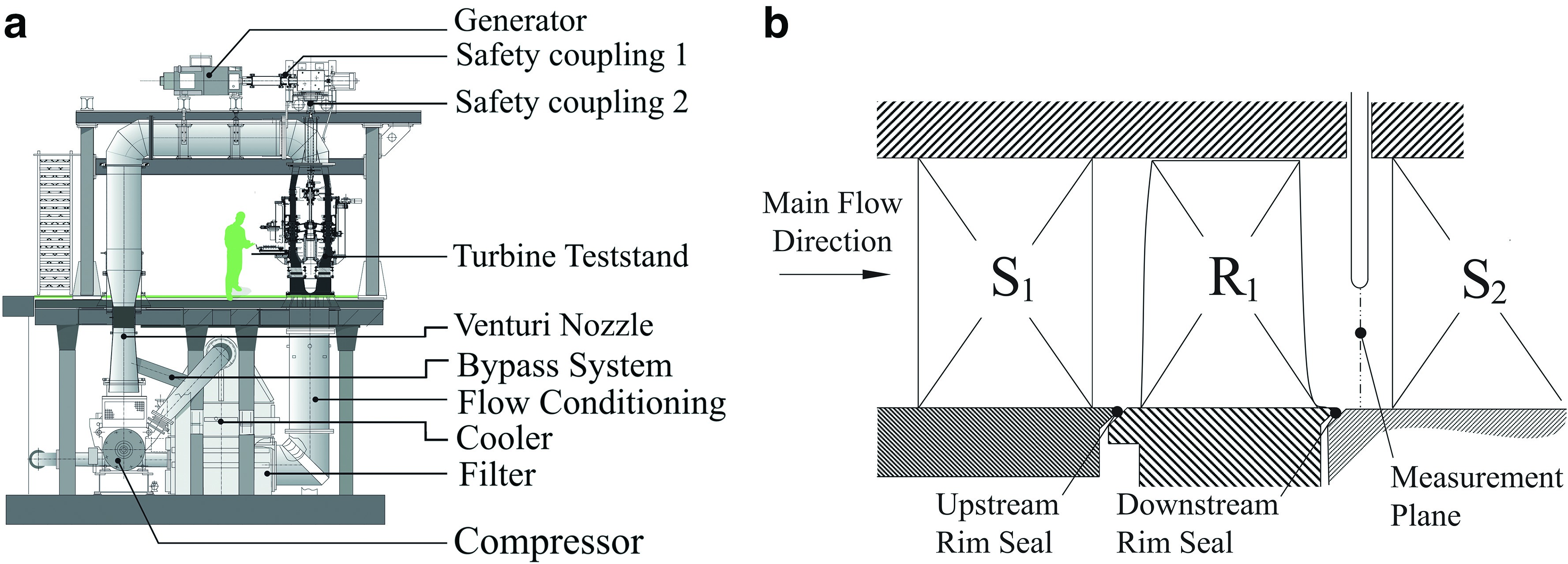
The highly loaded turbine operates at moderate speeds and low temperatures. The rotational speed of the turbine is kept constant by a DC generator with an accuracy of ±0.02% (±0.5 rpm). Furthermore, the turbine inlet total temperature is maintained constant with an accuracy of ±0.3 K, with the use of a heat exchanger at the inlet. A detailed description of the turbine design can be found in 3. The main operational parameters of the facility are summarized in Table 1. For this work, measurements are performed at the exit of the rotor, over one stator pitch. A total of 41 traverses are performed in the circumferential direction (every 2.5% of the pitch), while 37 radial positions are taken per traverse. The radial points are clustered towards hub and tip and cover a range from 7 to 99.5% span. The measurement grid of total 1,517 points required approximately four hours for FRAP-4S. The same measurements for FRAP-2S need close to 9.5 hours, due to V4S operation. The FRAP data were acquired with 200 kHz sampling rate and 24 Bit resolution. This resulted in a total of 105 samples per rotor blade passage. An ensemble of 85 revolutions are then kept for phase-lock averaging and to perform statistically reliable analysis.

Table 1.

Geometrical features and operating conditions of 1.5 stage axial turbine LISA.

Rotational Speed	2700 ± 0.5	[rpm]
Pressure ratio	1.65 ± 0.1%	[-]
Inlet total temperature	326.7 ± 0.3	[K]
Capacity	150.9 ± 0.1	[kg⋅Ks⋅bar]
Aspect ratio (S1/R1/S2)	0.89/1.21/0.83	[-]
Blade count (S1/R1/S2)	36/42/36	[-]
Mach at exit (S1/R1/S2)	0.53/0.27/0.48	[-]
Chord based Reynolds number	7.10/3.80/5.10	[×105]

Results and discussion

The present work focuses on the applicability of multi-sensor fast response aerodynamic probes for turbomachinery applications. First, the time-averaged measurement performance of the FRAP-4S is compared to the traditional 5 HP. Subsequently, the turbulent flow-field distribution at rotor exit is discussed in detail.

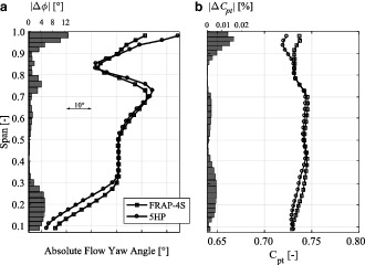
Figure 7 shows the span-wise distribution of the area- and circumferentially averaged yaw angle and C_pt, measured with the 5 HP and FRAP-4S at rotor exit. The flow-field can be divided in four distinct regions: the tip leakage vortex region from 100 to 90% span, the tip passage vortex region from 90 to 70% span, the pure blade wake region from 70 to 40% span and finally the region affected by the presence of the hub secondary flow structures ranging from 40 to 10% span. The absolute deviation between FRAP-4S and 5 HP measurements are shown as bar charts at the left of each graph. It can be seen that the deviations in measured yaw angles are maximum in the regions of highly skewed flow, which can be attributed to the larger sensing area and flow blockage surface of the FRAP-4S compared to the 5 HP. Interestingly, in the mid-span region, from 30 to 70% span, the 5 HP and FRAP-4S measurements match remarkably well. In the uniform region from 30–50% span the difference is null, while a slight increase is shown as soon as the gradient appears at 60% span. Similarly, the steep gradient at 75% span is causing the overshoot in the deviation from pneumatic data. Looking now at the C_pt profiles, similar to yaw angle measurements the largest deviations occur in the regions affected by the secondary flow structures with best agreement found around mid-span. The differences on average are close to 0.5%, while at tip deviation from 5 HP as high as 2.3% can be seen.

Figure 7.

Area- and circumferentially averaged (a) absolute yaw flow angle and (b) total pressure coefficient.

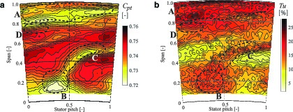
The time-averaged area plots of the measured total pressure coefficient and anisotropic turbulence are shown on Figure 8, providing an overview of the flow-field distribution across one stator pitch at the exit of the rotor. In Figure 8, the large total pressure deficit region (A) ranging from 75 to 100% span is directly related to the presence of the rotor tip leakage and tip passage vortices. The unshrouded rotor blades, allow the expansion of the main flow across the rotor tip gap from the pressure to the suction side, which then rolls-up into the rotor tip passage vortex. In that region the highest levels of unsteadiness can be found with turbulence intensity levels up to 25% (Figure 8). On Figure 8, close to the hub centred at 15% span and 35% pitch, the trace of the corner and hub passage vortices can be seen. This interaction can be identified as a local total pressure loss-core, which results in a second region (B) of increased stochastic unsteadiness as seen on Figure 8. The third major region (C) of total pressure deficit and elevated turbulence intensity is located from 40 to 60% span and spread over 50% of the stator pitch. This signature is most probably related to the stator wake structure, periodically chopped by the incoming rotor blade.

Figure 8.

Time averaged (a) total pressure coefficient and (b) anisotropic turbulence intensity measured with FRAP-4S. Observer looks upstream.

The discussion will now focus on the turbulent flow quantities and the contribution of each velocity vector to the measured level of turbulence intensity. To evaluate how the turbulence isotropy assumption holds; a comparison is performed between isotropic and non-isotropic turbulence levels. To compute isotropic Tu_iso only the streamwise fluctuating component is used, based on Equation 5.

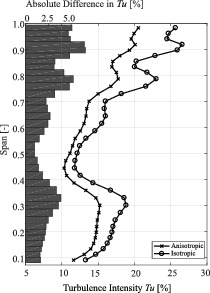
In Figure 9, the area- and circumferentially averaged turbulence intensity profile are provided. It is clear that at this position at the exit of the rotor the assumption of isotropic turbulence does not hold. A constant offset of approximatelly 2.5% difference across the entire span can be seen, while in the regions affected by the presence of the tip passage and tip leakage vorticies at 77 and 90% span the isotropic turbulence intensity tends to overestimate levels of stocastic unsteadiness by more than 5%. It should be noted that at midspan the istropic turbulence intensity shows the lowest deviation of 1% compared to the anisotropic formulation as the contribution to the stochastic unsteadiness comes primarly form the freesteam turbulence. It can be concluded that the crosswise velocity fluctuations are in general significantly lower compared to the streamwise direction.

Figure 9.

Area- and circumferentially averaged turbulence measured with FRAP-4S.

The time-resolved turbulence intensity across the circumference is now analysed in detail at the rotor exit at 77% span and over three rotor blade passing periods. Figure 10 presents the time-space plots for C_pt (a) anisotropic turbulence (b), as well as the Degree of Anisotropy (DA) as defined in Equation 6.

Figure 10.

Time-space diagrams for total pressure coefficient (a), anisotropic turbulence (b) and Degree of Anisotropy DA (c) at 77% span.

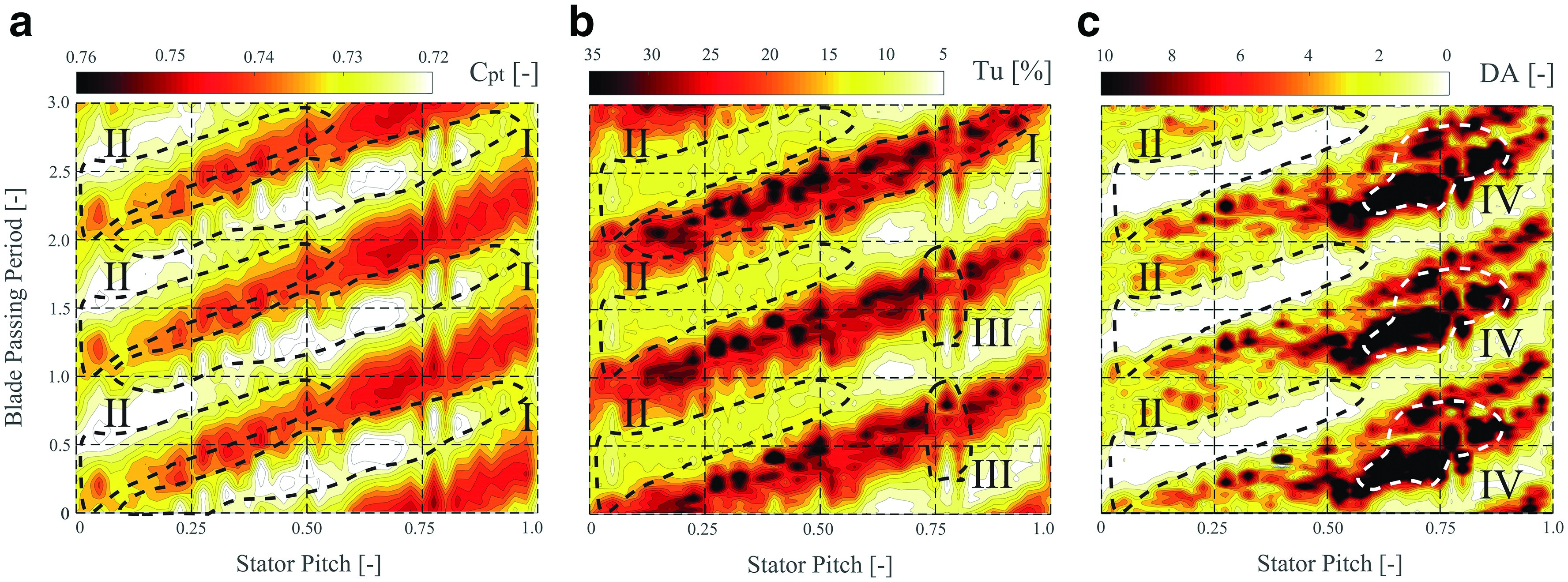
The DA is used to quantify the departure from isotropy by comparing the turbulent crosswise (v and w) and streamwise (u) velocity components. As shown in Figure 10 and Figure 10, the presence of the rotor tip passage vortex translates into alternating regions of elevated turbulence intensity and total pressure loss. In region I, where the tip passage vortex is located, the anisotropic turbulence levels are close to 25%.

The isotropic turbulence formulation leads to larger values, up to more than 40% in turbulence intensity (not shown here). Furthermore, in the free-stream zone (II), the turbulence is under-predicted in the isotropic case compared to the non-isotropic showing turbulence intensities ranging from 5 to 10%. In the third region of interest (III) a spike-like variation of the turbulence levels can be seen and is attributed to the ingestion of the upstream stator wake by the tip passage vortex. The DA plotted in Figure 10 highlights the strong peak-to-peak variations between the freestream and the secondary flow regions.

In the DA distribution two regions are highlighted, the free-stream region (II) where the DA decreases down to a minimum value of 0.28 and the region IV, where the stream wise fluctuations are ten times more intense than in the cross-wise direction. In region II the flow is only weakly affected by secondary flows, resulting in moderate average total pressure and turbulence levels (Figure 8, Figure 8 zone D). In that zone, the crosswise turbulence components tend to be nearly 4 times higher, compared to the stream-wise direction.

In order to gain more insight into the contribution of each velocity components to the overall turbulence, the temporal variaton of turbulence intensity (non- and isotropic) and the percentage contribution of each velocity components over three blade passing events are depicted in Figure 11 and Figure 11, respectively, for a measurement point located at 77% span and 0.2 stator pitch. Figure 11 confirms that the assumption of isotropic turbulence does not hold in the context of rotating machinery flows.

Figure 11.

Turbulence intensity (a) and contribution of each velocity component to the overall turbulence level (b) at 77% span and 0.2 stator pitch.

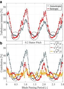
The isotropic turbulence tends to overstimate the turbulence levels found in the secondary flow structures, wheras in regions weakly affected by secondary flow structures the opposite is true. This observation is in line with the work presented in 25, even though their survey was conducted at the exit of a stator stage. As shown in Figure 11, it can be observed that the contribution of the both crosswise terms to the freestream turbulence tends to be of the same order of magnitude, whereas across the tip passage vortex the meridional components show up to 10% (in absolute values) more contribution than the vertical component.

Conclusions

A novel 4-sensor fast response aerodynamic probe with a hemispherical tip diameter of 4 mm was successfully developed, calibrated and tested in a high-pressure axial turbine research facility. The probe demonstrated its reliability to perform accurate time-averaged and resolved measurements in the challenging environment of this highly loaded, low aspect ratio turbine configuration. The main conclusions drawn from the presented work are summarized below:

Nomenclature