
Introduction
Conventional power sources are anticipated to lose relevance due to a significant increase of renewables but will retain its major role in the overall energy mix. Besides advantages for the environment, it is worth noting that renewables will also become the best economical choice for most countries. Thus, two thirds of the global investment for power plants is expected to be spent on renewable power production (International Energy Agency (IEA), 2017). Furthermore, renewables will account for 40% of the total increase in primary energy sources (U.S. Energy Information Administration, 2017; British Petroleum (BP), 2018). While the proportion of oil and coal is predicted to decline, the use of natural gas is anticipated to increase significantly by 45% between today and 2040 (International Energy Agency (IEA), 2017). In order to meet the increased demand for natural gas, new exploration and production techniques need to be developed (International Energy Agency (IEA), 2014). But what actually causes natural gas to gain importance in the next decades? There are numerous obvious reasons such as efficiency and environmental legislations like emission limits. A further reason is that power production by gas turbines plays a key role in the process of implementing a large share of renewables. Especially small- to mid-sized gas turbines are able to quickly change their load as mentioned by Wiedermann (2010). Volatilities of renewable power production cause fluctuations that need to be compensated in order to guarantee a stable public grid frequency. Besides compensation by changing the load in terms of secondary control, gas turbines also act as primary control systems. Due to these properties, gas turbines are the ideal counterpart to renewables and are thus a sustainable technology as mentioned by Sinn (2017). In order to prepare gas turbines for the challenges of tomorrow, reduction of emissions, increase of flexibility, efficiency, and reliability is of high technical relevance. To fulfil their new role, modern gas turbines need to be able to perform fast load changes in a large operating window. Load flexibility is hence an essential feature for meeting the requirements of tomorrow and therefore frequently subject of various studies. Note, load changes in gas turbines are achieved by adjusting the fuel supply as mentioned by Sattelmayer (2010). A simultaneous reduction of the air mass flow can be accomplished to a certain degree by adjusting the compressor’s guide vanes as discussed by Möning and Waltke (2010). Once the minimum air mass flow is reached, a further reduction in load leads to a decrease of the global fuel-to-air ratio and colder flames. Note that nitrogen oxide (NOx) is mainly a function of temperature according to the Arrhenius law. The key difference between NOx and carbon dioxide (CO) is that the latter is an intermediate species in hydrocarbon-based combustion. CO usually reaches a maximum within the flame that is orders of magnitude higher than the limits given by emission legislations. The burnout of CO is hence a mandatory step to reduce CO emissions. Super-equilibrium CO may occur in cold conditions as the temperature-sensitive burnout of CO cannot be completed. Under conditions that show sufficiently high temperatures, the burnout is fast and the reactive flow quickly approaches equilibrium. Below a specific flame temperature, the equilibrium state can no longer be reached, and CO emissions rise sharply. The lower limit of fuel reduction is given by the lean blowout event. The contrary trends in CO and NOx as a function of Tad may lead to a narrow range of possible operating conditions. An example is given by Lefebvre and Ballal (Lefebvre and Ballal, 2010) who stated that flame temperatures between 1670 K and 1900 K are ideal to obtain NOx values below 15 ppmv and CO values below 25 ppmv. There are several strategies for augmenting the operating window towards lower loads while keeping CO emissions below a certain threshold. For instance, an adjustable combustor geometry can be employed to control the flame temperature by air staging (Lefebvre and Ballal, 2010). The strategy is to increase air mass flow at full load to cool the burnout area and prevent the oxidation of dinitrogen (N2) to NOx. At part-load conditions, air is reduced to increase the temperature in order to ensure CO burnout. However, the operation of a variable combustor geometry is complex and its industrial employment is rare (Lefebvre and Ballal, 2010). A more practical approach to extend the range of possible operating conditions is to stage fuel instead of air. Fuel staging is the redistribution of fuel supply to exploit various mechanisms for the emission-safe operation of gas turbines at part load. Technical implementations of fuel staging are widely used in industry and are of high relevance for the present work. An overview of different fuel-staging strategies is given by Sattelmayer (2010). Technical concepts are often based on one or both of the following two mechanisms:
In order to accomplish full burnout at part-load conditions, burners that operate below the lean blowout limit need to be ignited by pilots. Piloting is based on the phenomenon of self-ignition temperatures that are usually far below the adiabatic flame temperature (Sattelmayer, 2010).
In multi-burner systems, it may be reasonable to supply only a fraction of all burners with fuel leading to locally increased temperatures and faster burnout downstream of the group of active burners. Note, quenching effects may occur at the interface to cold, inactive burners.
In this work, a modeling strategy is introduced that is able to capture both mechanisms. The model is based on a combustion model published by the authors in Klarmann, Sattelmayer, Geng et al. (2016) and Klarmann, Sattelmayer, Zoller et al. (2016). The combustion model is an extended version of the Flamelet Generated Manifold (FGM) and designed to achieve high accuracy in low-reactive conditions in which effects like flame stretch and/or heat loss may be relevant. It is important to note that a combustion model that is based on the flamelet assumption can only predict elevated CO emissions if the turbulent flame brush thickness is in the magnitude order of the combustion chamber or if the flamelets fluctutate to the outlet. As both assumptions are not realistic, it can be argued that the flamelet assumption is not valid when CO emissions occur. Furthermore, the prediction of CO using FGM requires excessive model tuning as it is shown by Goldin et al. (2012a, b). The authors concluded that FGM drastically overestimates the CO source term during burnout. Another attempt to numerically predict CO using CFD methods is done by Wegner et al. (2011), where CO is described by a transport equation that is decoupled from the combustion model. Within the turbulent flame brush, CO is initialized using the maximum value of CO at a predefined reaction progress. CO peak value is determined by one-dimensional simulations based on detailed chemistry. The idea of separating the time scales of combustion and burnout is adopted in the present work. The CO model was firstly introduced and validated in an atmospheric single-burner test rig in Klarmann et al. (2018). In the following, this modeling strategy is extended to consider quenching effects that are demonstrated to play an important role in predicting CO emissions. Validation is performed using two multi-burner cases that differ in terms of pressure and the way fuel is staged in part load operation.
Methodology
In the following, the proposed CO-modeling approach is introduced. It is based on the combustion model that was published by the authors in Klarmann, Sattelmayer, Geng et al. (2016) and Klarmann, Sattelmayer, Zoller et al. (2016). We propose the employment of an isolated transport equation to describe the Favre-averaged mass fraction of CO:
The strategy for closing this equation is based on the spatial division into multiple zones in a way that is illustrated in Figure 1. A Lagrangian observer is shown that travels on a trajectory through a combustor and passes several regions. The observer’s position determines the employed sub model for CO. In the lower half of Figure 1, a qualitative profile of CO as a function of the Lagrangian observer’s travelled distance is shown. The continuous line represents CO predicted by the combustion model. As the Favre-averaged reaction progress
Figure 1.
Illustration of the divide-and-conquer approach using a Lagrangian observer traveling trough a combustion chamber (adapted from Klarmann et al. [15]).
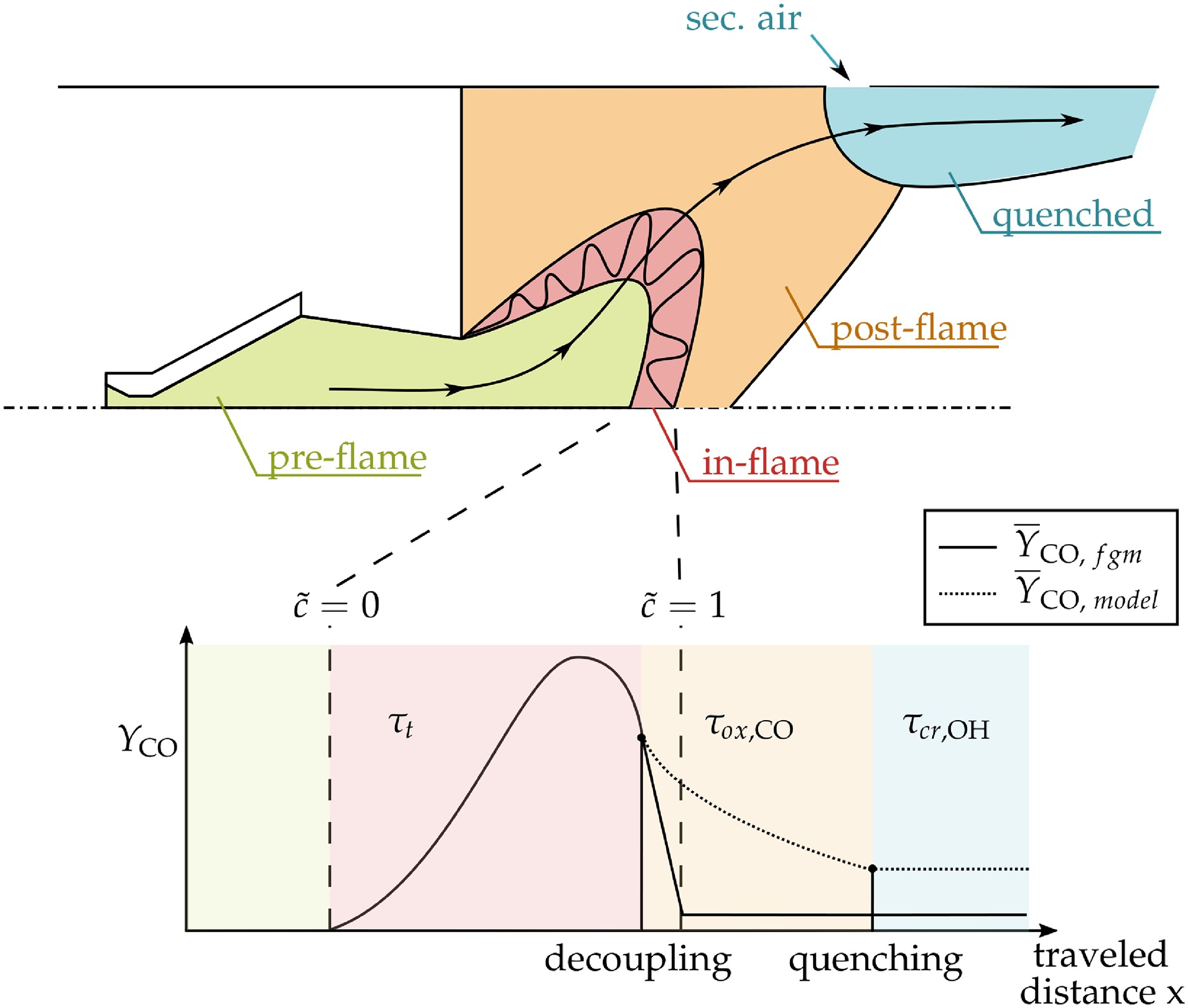
After CO is not described by the flamelet-based species trajectories (continuous line), CO oxidation becomes slower due to the absence of the flamelet’s radical pool. Moreover, the post-flame model presented in this work loses its validity in situations in which the equivalence ratio is significantly decreased. In summary, four different regions of different modeling are defined:
pre-flame zone: CO chemistry is negligibly small and we do not consider any source terms here.
in-flame zone: Within the turbulent flame brush, chemical time scales are assumed to be smaller than turbulent time scales. We hence consider turbulent mixing to be the limiting mechanism and CO is described by flamelets. As shown by the authors in Klarmann et al. (2018, 2019), it is important to consider flame stretch as well as heat loss.
post-flame zone: The interface between in- and post-flame zone is defined by the point at which the turbulent time scales are not the limiting factor anymore as chemical time scales become dominating. Details regarding modeling of the time scales is provided in the following.
quenched zone: In the potential situation of lean quenching, the equivalence ratio is low and the chemical rates are negligibly small. As argued in the following, this region is dominated by the creation time scale of hydroxyl (OH).
Post-flame zone
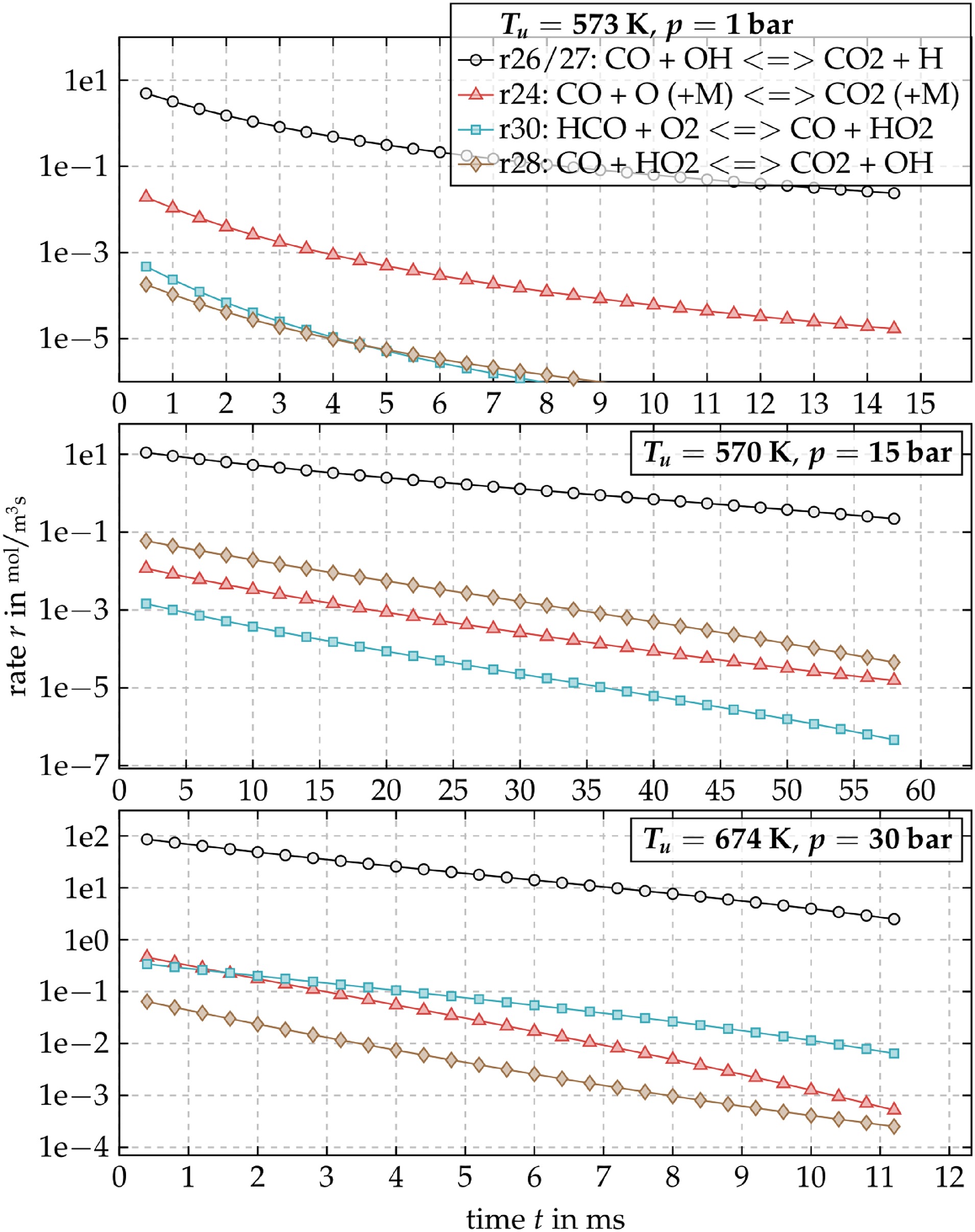
As it was shown in experiments by our group in Klarmann et al. (2019), freely propagating flamelets are not suitable to describe chemistry behind the turbulent flame brush. In general, burnout chemistry of CO can be described using a single reaction equation as mentioned by Turns (2000):
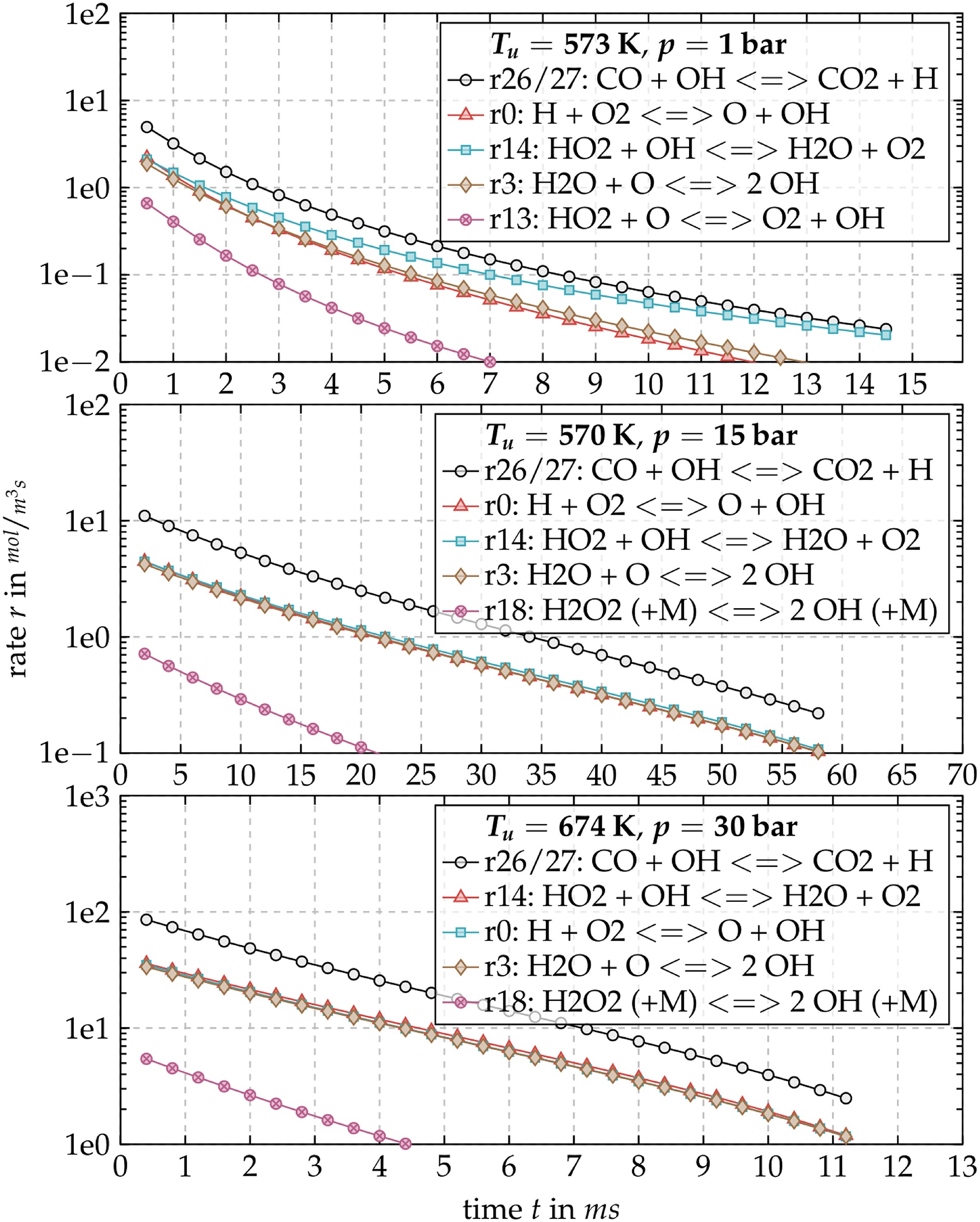
Reaction rates that are obtained from a zero-dimensional reactor simulation (Cantera (Goodwin et al., 2015)) are shown in Figure 2 at three different constant pressure conditions for an equivalence ratio of
Figure 2.
The four most relevant CO reactions in the late burnout (constant pressure reactor at an equivalence ratio of 0.3 calculated using Cantera [18]).
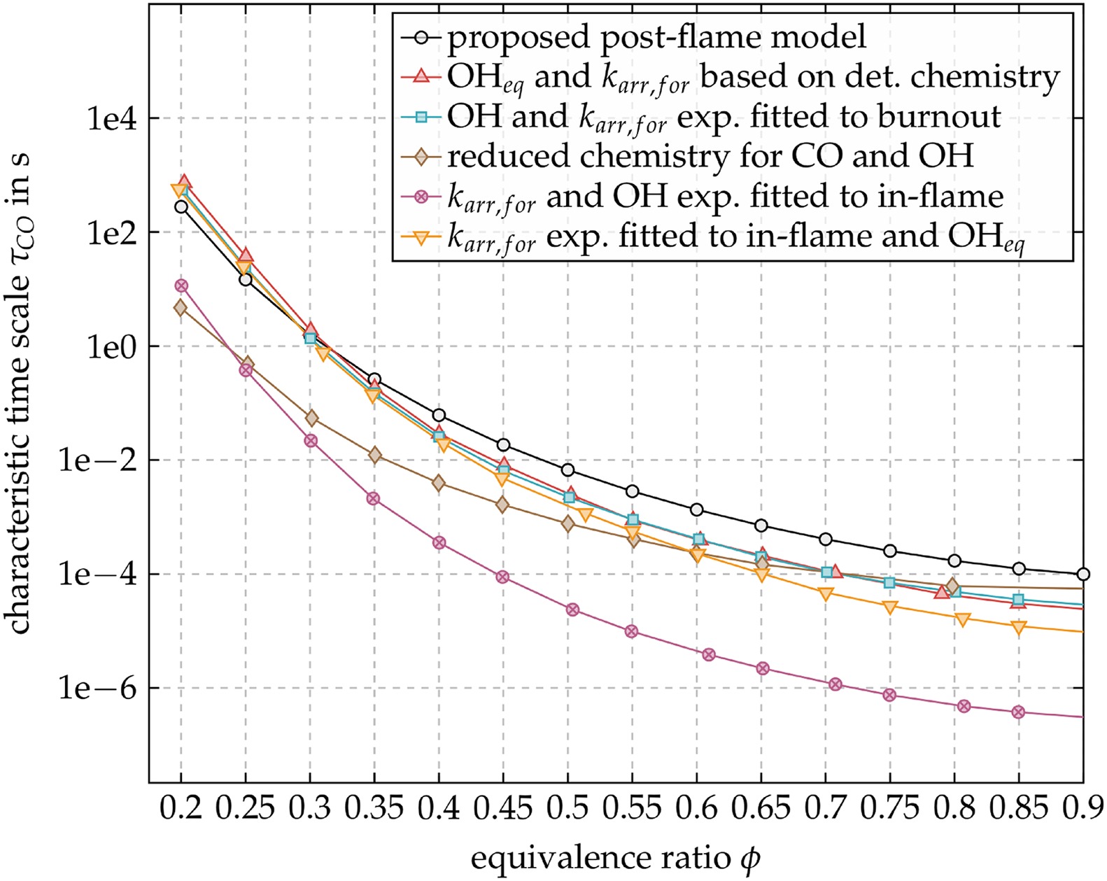
In the present work, the equilibrium of OH is determined using Galway 1.3 (Metcalfe et al., 2013) kinetics. Furthermore,
Figure 3.
CO burnout time scales for different strategies of considering OH (reprinted and adapted from Flagan and Seinfeld [22]).
In order to prove the validity of the proposed post-flame model, we conducted atmospheric experiments. The geometry is depicted in Figure 4. Details to the experiment are show in Table 1. CO is measured by using a water-cooled probe at the indicated locations. Note that CO is measured and averaged at three different radii for each distance. The CO concentrations are used to derive source terms by using residence times between each distance that are retrieved from a corresponding CFD simulation (Fluent v.18 (ANSYS Inc., 2014)). In Figure 5, the resulting experimental CO source terms as a function of distance to the front plate are plotted. Moreover, experimental and numerical source terms are compared for two different adiabatic flame temperatures. The numerical CO source terms are calculated by using the proposed post-flame model (cf. Equation 3). After reaching a distance of 224.5 mm, the post-flame model prediction and the experiments are in good agreement. It is apparent that the transition from the in- to the post-flame zone should be predicted to occur between 199 mm and 224.5 mm. In addition, Figure 5 shows CO source terms obtained from a constant pressure reactor (blue dashed line) and from a freely-propagating flamelet (brown dashed line) at the corresponding reaction progress. Note that the experimental reaction progress source term can be derived from the measured carbon dioxide (CO2) and CO concentrations. Both simulations drastically underestimate the source term due to the already discussed situation of elevated OH that is able to quickly burn out CO.
Figure 4.
Illustration of the atmospheric single-burner test rig with indicated post-flame measurement locations.
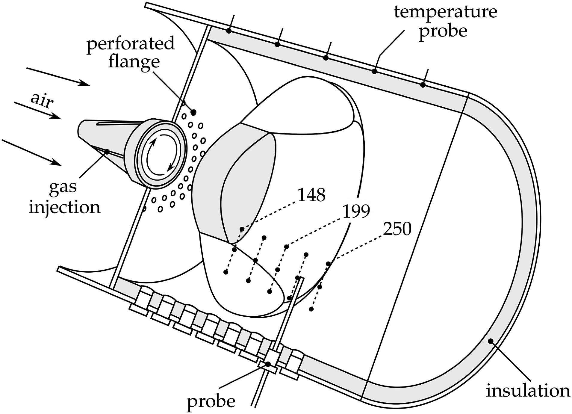
Table 1.
Experiment's boundary conditions.

Modeling the transition to post-flame
Models for closing CO within the flame and downstream of the turbulent flame brush are introduced in the previous sections. An additional model is needed to predict the reaction progress at which the transition from in- to post-flame occurs. A transition model is proposed by Wegner et al. (2011) in which CO is set to the maximum value of CO occurring in the flame front at a predefined reaction progress. This idea is simple and robust but has a major simplification as it neglects the potential oxidation of CO within the turbulent flame brush before decoupling occurs. As demonstrated in the previous section, the flamelet-based oxidation of CO is usually significantly stronger than the burnout chemistry. Hence, a transition model is proposed that allows a fully flamelet-based closure in conditions in which the flamelet assumption is continuously valid during CO burnout. A suitable model for predicting the transition event needs to be based on a single criterion that unambiguously evaluates the validity of both the in- and the post-flame model. The criterion that is proposed in the following is modeled by comparing time scales. The in-flame model uses the assumption that all chemical time scales are faster than turbulent time scales. Furthermore, the post-flame zone is dominated by the slow burnout chemistry. The transition model in the present work is thus based on a Damköhler number that compares turbulent and chemical time scales:
Both time scales are specified in the following. A reasonable choice that we identified for the chemical scale is the time of oxidizing CO within the turbulent flame brush. It is approximated by assuming a bimolecular reaction (cf. Turns, 2000):
The turbulent time scale can be interpreted as a characteristic time for micro-mixing and reads
In the context of RANS simulations, k and
Modeling lean quenching
In order to guarantee low emissions at part load, gas turbines usually employ fuel staging concepts. Lean streaks may occur due to inactive burners, leakage air from sealings, and cooling air from liners. The mechanism of diluting the reactive flow to a level in which the reaction rates decrease to zero is denoted as lean quenching. Note that the combustion model, and consequently the in-flame model, are inherently able to consider lean quenching effects, as premixed counterflow flamelets can be calculated even for mixture fractions that are close to zero.
The proposed post-flame model is based on the assumption that OH is in equilibrium during burnout implying that the recreation of OH is always faster than the burnout of CO. A numerical analysis of this simplification is demonstrated in Figure 6. The left y-axis shows the burnout time as a function of adiabatic flame temperature
Figure 6.
Temperature dependent burnout time and ratio of OH creation to CO oxidation (constant pressure reactor at p = 15 bar, calculated using Galway 1.3 [20] and Cantera [18]).
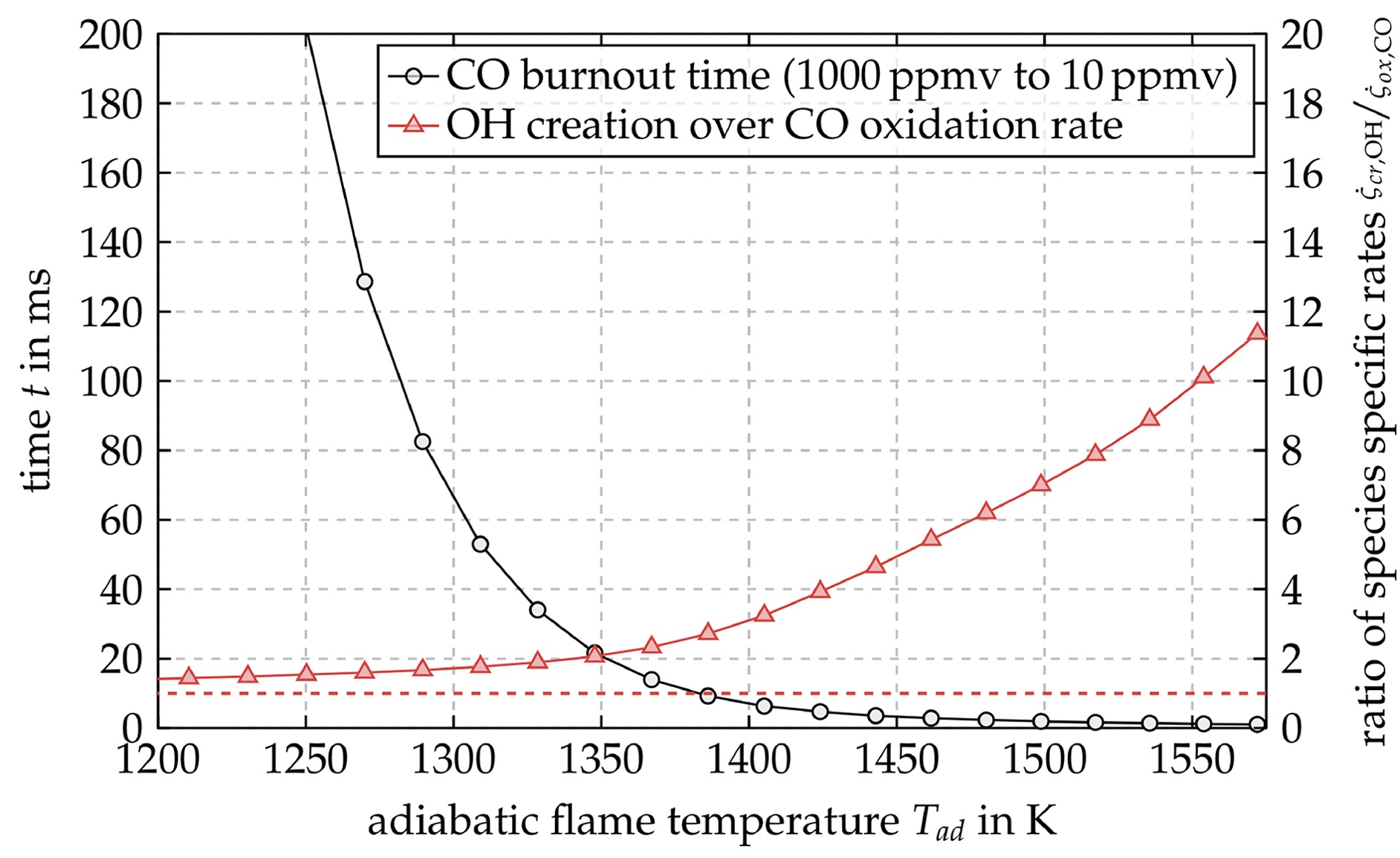
Figure 7.
Five most relevant OH reactions in the late burnout (constant pressure reactor at an equivalence ratio of 0.3, calculated using Galway 1.3 [20] and Cantera [18]).
In the following, it is assumed that all reactants on the left-hand side of this set of equations are in equilibrium and that solely the forward reaction is relevant. Note, the burnout of CO does not significantly alter dioxygen (O2) and water (H2O) as both species are available in abundance. Fast time scales can be assumed for the following radicals: Hydrogen (H), oxygen (O), and hydroperoxyl (HO2). This leads to a model that allows to tabulate the OH creation rate
A critical value of unity is used throughout the present work as this value implies the point at which CO oxidation exceeds OH creation.
Validation
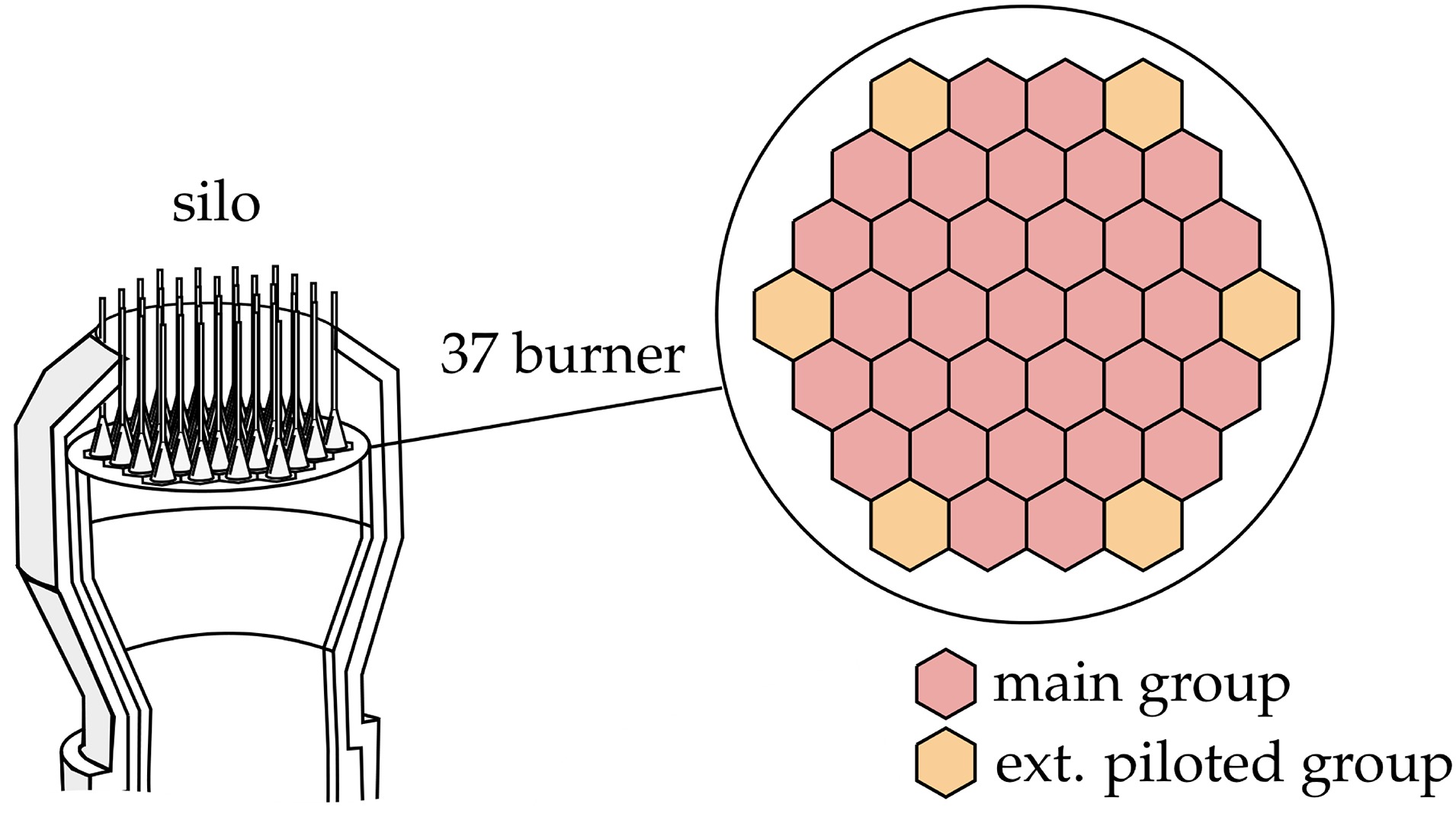
The validation of two multi-burner cases that employ fuel staging concepts are presented in the following. Both cases use the GT11N silo combustor geometry that comprises 37 burners as illustrated in Figure 8. The first validation case is a down-scaled, atmospheric model of the GT11N. In addition, validation of a full-scale GT11N in field operation is presented. An overview of the numerical setups is given by Table 2. Both cases operate under part-load conditions in which solely a part of the total amount of burners is active. Multiple stages exist that differ in their number of active burners. A specified group of burners is switched off during the transition to a colder stage. By reducing the power to part load conditions, several stages are passed and the number of burners is successively reduced. The decisive difference between both fuel staging scenarios is the way fuel is reduced before a group of burners is switched off:
Figure 8.
Illustration of the GT11N (inspired by Vorontsov et al. [27]) emphasizing the employed fuel staging concept of the atmospheric case.
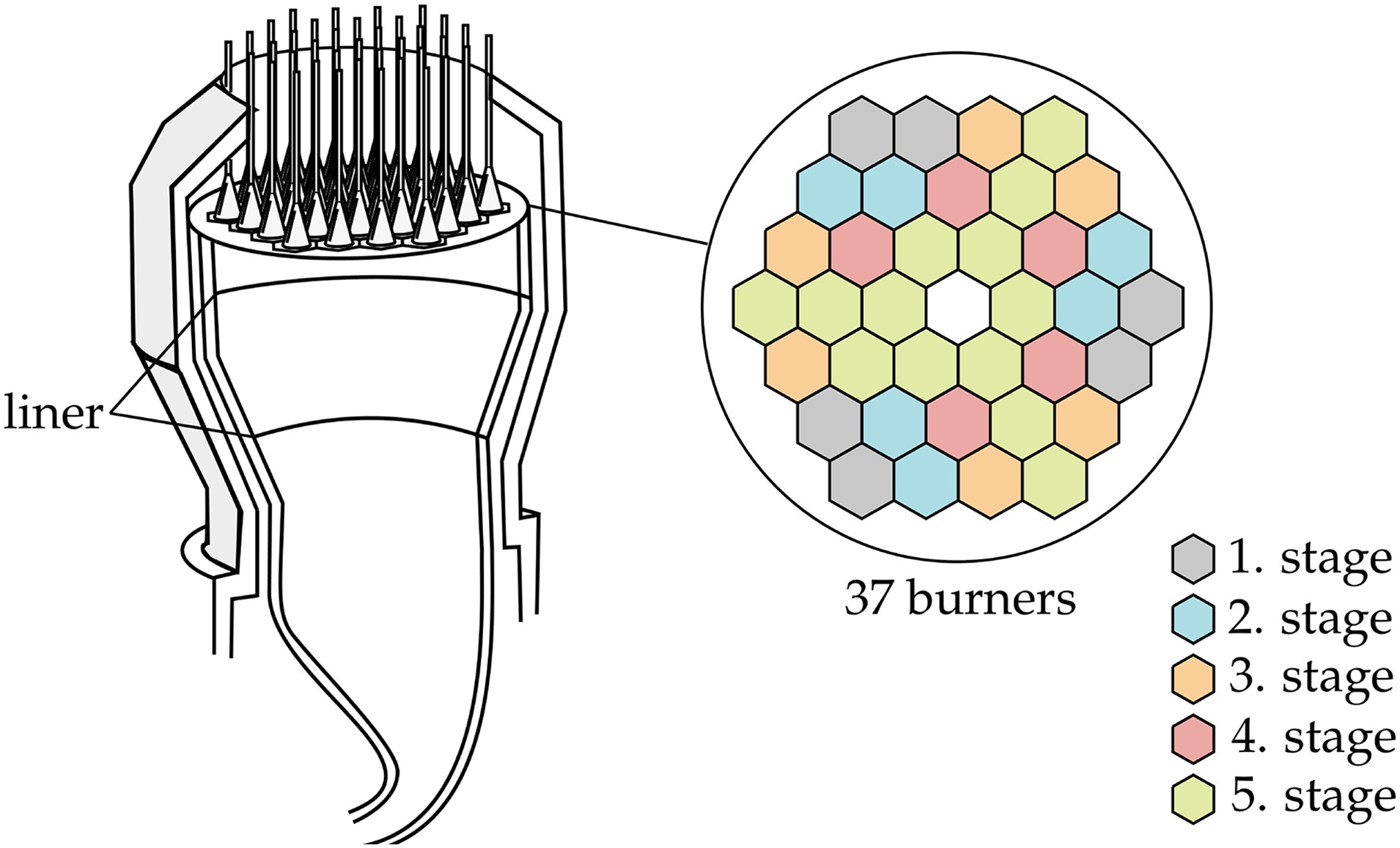
Table 2.
Setup for the multi-burner cases.
Atmospheric GT11N model: A group of burners is ramped down from reference conditions to pure air. Variation of load during a stage is conducted by solely changing the fuel supply of the specific group that is intended to get switched off.
High-pressure GT11N in field operation: The reduction of load is accomplished by decreasing the fuel supply for all active burners. This can be done until CO emissions increase to a specific limit. When this limit is reached, a group of burners that operates at stable conditions is abruptly switched off. The fuel surplus from the switched-off burners is redistributed to the remaining group of active burners leading to a drop in CO emissions.
All introduced models are implemented in Fluent v.18 (ANSYS Inc., 2014). The shown results are retrieved from a steady, pressure-based RANS CFD simulation.
Atmospheric GT11N model
The validation of a down-scaled, atmospheric model of the GT11N is presented in the following. The experimental data is retrieved from an unpublished, company-internal measurement study that was conducted in order to find reasonable fuel staging strategies for silo combustors. In the report, the optimal concept for part-load operation is investigated in terms of how the burners should be grouped and in which order the groups should be phased out when reducing the load. The burner grouping is depicted in Figure 8 (illustration inspired by Vorontsov et al., 2009). It is important to note that this burner grouping is not a reasonable strategy for real gas turbines and should be interpreted as a benchmark test in terms of CO emissions. For example, the last group of burners that remains active for the coldest conditions (stage 5) is the most critical group. A reasonable strategy would be to locate the active burners of stage 5 in a way that the number of cold neighbours is minimized. However, the burners of stage 5 are far apart from each other, have many cold neighbours, and are hence not optimal in terms of CO emissions in part load.
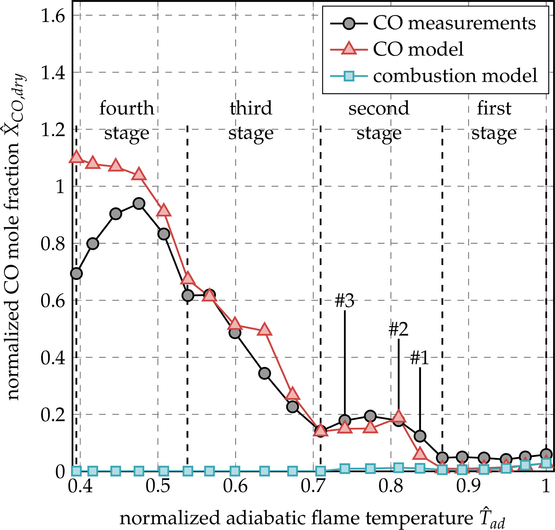
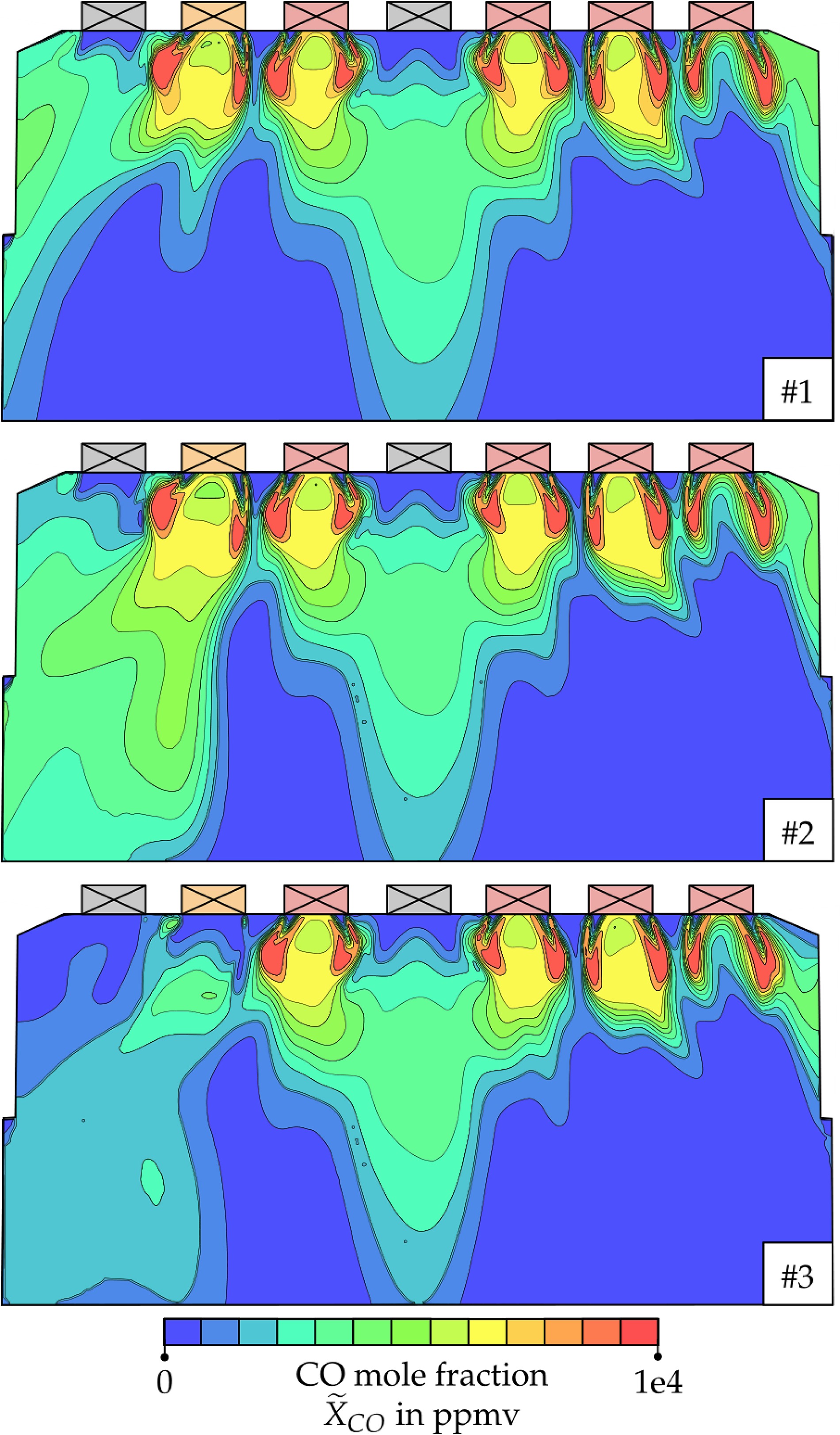
Unfortunately, the exact geometry of the atmospheric model of the GT11N is not available. However, the geometry of the full-size GT11N is employed and geometrically scaled down to fit the combustion chamber’s diameter of the atmospheric model. The geometry comprises the plenum, all burners, the combustion chamber, and the transition piece. CO mole fraction
High-pressure GT11N in field operation
The burner layout that is used in the high-pressure case is illustrated in Figure 11. 31 single switchable burners are belonging to the main group (red burners). The central burner is not active for the operating points that are considered in this study. Six burners of the piloted group (orange burners) are located in each corner. Piloted burners are supplied with substantially less fuel than burners that belong to the main group. Figure 12 demonstrates the interaction between the two groups. The first contour plot shows the laminar flame velocity

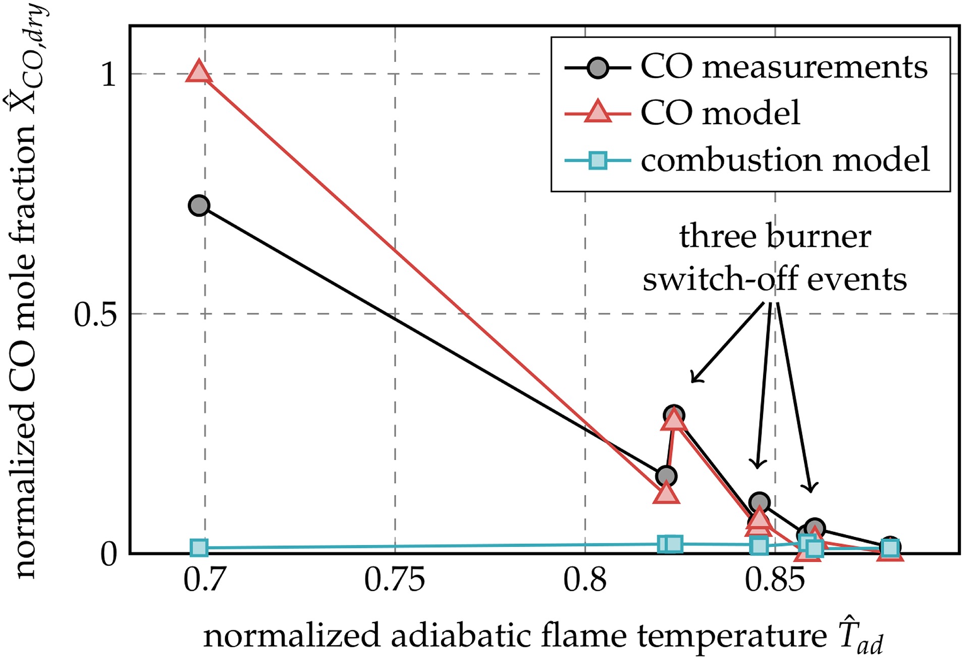
Validation is performed by comparing modeled with measured CO emissions as function of adiabatic flame temperature
Summary and discussion
Model validation for the numerical prediction of CO emissions in gas turbine combustors featuring multiple burners operating under part load conditions is presented in this paper. The modeling approach divides the domain in multiple regions and models each section differently. The model’s capacity to capture the following phenomena is demonstrated:
Typical behaviour of global CO emissions as a function of adiabatic flame temperature.
Piloting of premixed flames that are operated below the lean blow out limit.
Lean quenching of flames interacting with colder neighbours.
The modeling strategy is validated with CO emissions obtained by comparing numerical results to two different cases. An accurate prediction of the CO emissions without model tuning is achieved. Furthermore, the poor performance of the flamelet-based combustion model is demonstrated.
The modeling strategy of the present work exhibits two points of potential criticism that are addressed in the following:
The proposed modeling strategy is based on the comparison of time scales to predict the different zones in which the submodels are used. A valid criticism would be that the times scales should not be interpreted in an absolute way. For instance, the circumferential speed of eddies do not have an direct relationship to the CO burnout time but both quantities are compared to predict the transition from in- to post-flame. However, this approach should be reasonable if at least one of the following situations is true:
o
o There is a transition area in which the in- and post-flame model show similar source terms for CO reducing the error of a wrongly predicted decoupling event.
Turbulence-chemistry interaction is neglected during burnout. This is only valid if one or both of the two situations apply:
o CO burnout is slow and the variance of CO mass fraction is close to zero. This means that the PDF collapses to a singularity at the corresponding mean value and a PDF integration has no effect.
o Non-zero variances of CO mass fraction do not imperatively lead to the necessity of employing PDF integration. This is due to the fact that CO burnout chemistry can be assumed to behave linearly in the range of small variances.
Nomenclature
Latin
Reaction progress, -
Model specific Dammköhler number, -
Mixture fraction, -
Reaction rate constant
Turbulent kinetic energy,
Integral length scale,
Wall thickness,
Mass flow,
Proportionality exponent for stretch correction, -
Proportionality exponent for non-adiabatic correction, -
Pressure,
Reaction rate,
Laminar flame velocity,
Turbulent Schmidt Number, -
Time,
Temperature,
Velocity,
Spatial coordinate,
Mole fraction of species i,
Mass fraction of species i,