
Introduction
Rotating stall and surge are two main aerodynamic patterns in compressors, of which the latter has more detriment to the performance and physical integrity. Therefore, aerodynamic instability has been one of the main concerns in the compressor design. The researchers hope to take more effective measures to extend the stable operating range of compressors based on the mechanism of unstable flow processes. Aerodynamic instability has made great progress in the past decades, though accurate prediction and clear knowledge are still challenging for a new compressor (Day, 2016).
The surge was reported in the experimental investigation of compressors (Emmons et al., 1955) and was characterized by large-amplitude and low-frequency oscillation. The researchers have done much work to find the instability mechanisms. Earlier investigations described surge based on acoustic features (Pearson and Bowmer, 1949), then used high-responding transducers to record the flow velocity. For further understanding aerodynamic instabilities, many aerodynamic models were built to simulate the behaviours of the compression system. Moore and Greitzer (1976) built the lumped parameter model based on an axial compressor and found that the instability process relates to the pipe system. Fink (1988) and Tamaki (2008) applied this model to centrifugal compressors and conducted experiments with different pipe systems. Similar conclusions were drawn in the compression system including centrifugal compressors. With the development of computers and CFD algorithm, more three-dimensional (3D) models were built to study the detailed flow field. Jiang and Fu (2018) finished their 3D CFD code based on DES, and flow separation in a centrifugal compressor was investigated. However, it is time-consuming when running the 3D CFD models with full-annulus settings, especially for a multi-stage compressor. Therefore, some multi-dimensional models, such as Huang et al. (2019) and Dumas et al. (2015), were built to decrease the running time, the accuracy of which is acceptable.
Moreover, the flow details are distinctive in different configurations. For instance, rotating instabilities were reported in the research of Mathioudakis and Breugelmans (1985), and they usually exist in the blade rows with large tip clearance. Emmons et al. (1955) and Zheng and Liu (2015) found a special instability process called Two-Regime-Surge in the centrifugal compressor, which has never been reported in axial compressors. Lin (2023) further explained this phenomenon from the perspective of reverse flow and gave a quantitative analysis. The axial and centrifugal combined compressor is also commonly used and plays an important role in industrial facilities. However, the understanding of such compressors still needs to be improved. This paper focuses on a three-stage-axial and one-stage-centrifugal compressor and investigates its flow fields from choke to surge under off-design speed. The results from this work can support the aerodynamic instability design and transient force evaluation for the axial-centrifugal compressor.
Methodology
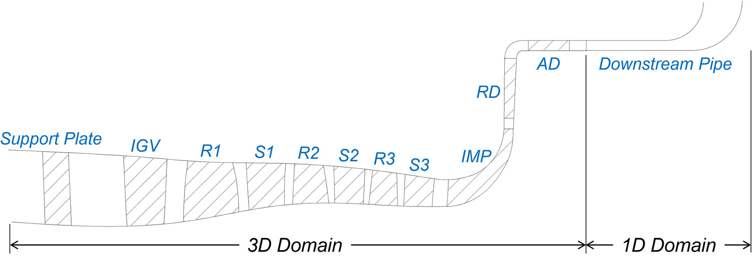
The meridional view of the three-stage-axial and one-stage-centrifugal compressor (3A1C) is shown in Figure 1. There are 10 blade rows, including inlet guide vanes (IGV) and outlet axial diffusers (AD). According to past findings, the pipe system deeply influences the aerodynamic phenomenon, and a multi-dimensional method is used in this paper to simulate the flow process. The pipe system, which mainly has a streamwise characteristic, is modelled by one-dimensional (1D) NS equations, while the complex flow in the compressor is simulated by 3D URANS equations. The one-dimensional-three-dimensional coupled method (1D–3D) was validated by experimental data and has a good accuracy in the surge simulation (Huang et al., 2019).
This method is described as follows. For the downstream 1D pipe system, the mass equation, momentum equation, and energy equation along the streamwise direction can be written as
where a is the sound speed, and the heat flux
where f is the Darcy friction coefficient, the 1D pipe flow model is a mature approach that has been widely studied and applied in many areas, such as internal combustion design (Galindo et al., 2008). For a compressor test rig, there usually is a plenum and valve. For the former, it can be assumed an isentropic flow and modelled as
where pp and ap denote the pressure and sound speed in the plenum, respectively. For the valve, it generates a back pressure, and its characteristic can be represented by the following equation
where Δp is the pressure loss and mv denotes the mass flow rate through the valve. Kv is a coefficient that represents the opening. The larger this value, the smaller the opening. For the interface between the 3D domain and 1D domain, When the air flows forward, the mass-averaged total pressure and total temperature are calculated from 3D domain outlet, which is given as the inlet boundary condition of the downstream pipe. The pipe outlet is the atmospheric conditions, and the 1D pipe flow can be solved by the characteristic line method. Finally, the static pressure at the pipe inlet can be obtained according to the 1D calculation, which is transferred to the upstream 3D outlet. Then 3D domain continues to the next physical time step. In contrast, when the air flows backward, the static pressure is transferred from 3D domain to 1D domain, and the total pressure and total temperature data are returned as the 3D domain outlet boundary after 1D calculation. More details concerning the theoretical model and solving process can refer to Huang et al. (2019).
The ANSYS CFX, which can be easily redeveloped and coupled with the 1D model written in Fortran, is selected as the solver of the 3D domain. Surge is the main focus of this paper, of which the frequency is low. It is time-consuming to run a complete surge cycle, so the model should be simplified to finish this work. Surge mainly exhibits a streamwise characteristic (Cumpsty, 2004), which means a single passage CFD model is acceptable. Figure 2 shows the mesh domain and grid distribution of 3A1C. For the 3D domain, the total pressure 101,325 Pa and total temperature 288.15 K are given as the inlet boundary condition, while the results of 1D model are given as the outlet boundary condition. The turbulence model is SST model. RANS cases were first run at choke condition, then 1D–3D URANS cases were run using the results of the steady case as the initial field, then we can move the operating point from choke to surge by changing Kv step by step. In the RANS model, the model between the rotor and stator is stage (mixing plane model in CFX), while it is transient rotor stator (sliding mesh model) in the 1D–3D run. Both numerical schemes for temporal and spatial discretization have two-order accuracy. The physical time step is 1 × 10⁻⁵ s in this work, about 16.6 steps per R1 passage. Moreover, the parameters of the pipe system should be given in the 1D model. The pipe length is 1.0 m, and the plenum volume is 1.5 × 10⁻⁴ m3 in this model.
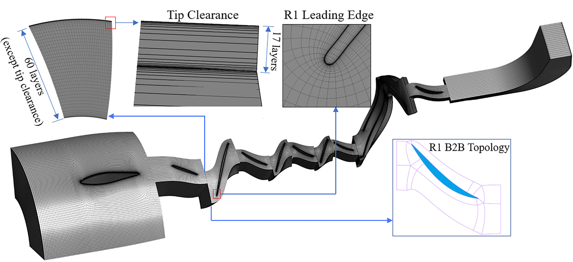
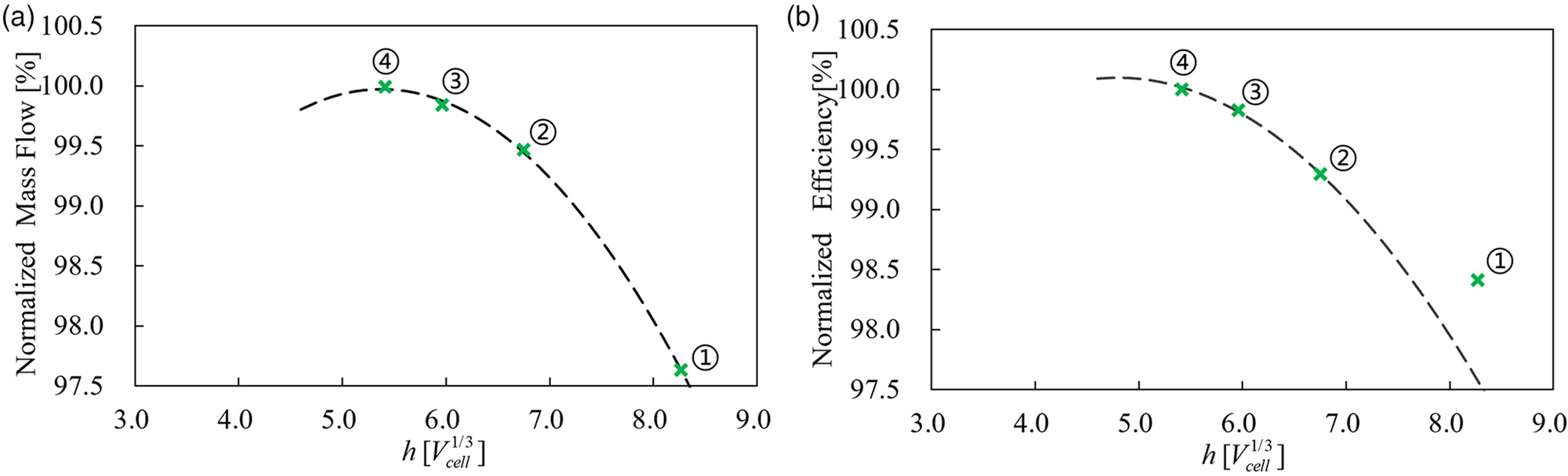
For a 3D numerical simulation, the mesh independence should be checked. Four mesh schemes, of which the nodes along three directions are added or reduced simultaneously, are calculated using the above RANS settings, and the results are shown in Figure 3. The y-axis of Figure 3a represents the choked mass flow at design speed, and Figure 3b is the efficiency trend at a fixed condition. The x-axis denotes the mesh scale h, which has the same order as 1/3 power of element volume vcell. The green symbols × denote CFD results, and the dashed lines are parabolic curves to fit the results. The choked mass flow and isentropic efficiency converge with the increased grid number. Mesh ④ has reached the peak point of parabolic curves, which is the final scheme used in this paper. As shown in Figure 2, there are 60 layers along the spanwise direction in the mainstream of each blade row, and there are 17 layers in the tip clearance region. The thickness of the first grid is 0.003 mm to ensure the Y+ requirement of SST model. The total grid number of 3D domain is 6.77 million. Fourteen days and 92 CPU cores are used to finish 27,000 physical time steps for a deep surge cycle using the above model, which is one order faster than a full-annulus model.
According to the theoretical analysis (Greitzer, 1976), the compression system with a small B parameter has a more complex instability process, in which the compressor may suffer from mild surge to deep surge instead of coming into deep surge directly. Therefore, an off-design speed is better for investigating unstable flow processes, and the unsteady simulation at 70% of the design speed was conducted in this paper.
Results and discussion
Compressor MAP
Figure 4 shows the MAP at 70% off-design speed, where the RANS results are marked with black triangles, and red rhombuses denote 1D–3D results. Apart from the CFD results, the experimental characteristic (marked as ×) is also plotted in this figure, which validates the accuracy of surge boundary. The pressure oscillation appeared gradually when the operating point moved from choke to surge. The rhombus denotes the average pressure and mass flow rate in a time window. Five working points, P1–P5, were run, and their transient mass flow rate histories are shown in Figure 5. The y-axis is the mass flow rate normalized by the choked mass flow. P1 has good convergence and is the stable condition. P2 has some oscillation, but the amplitude is quite small. With the close of the valve, a high-frequency oscillation appeared, as shown in P3 and P4, and the latter had a larger amplitude. Finally, the airflow broke down, and a deep surge happened.
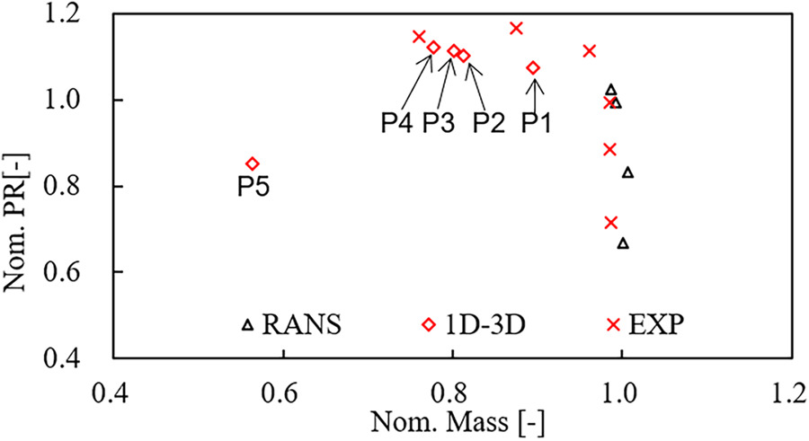
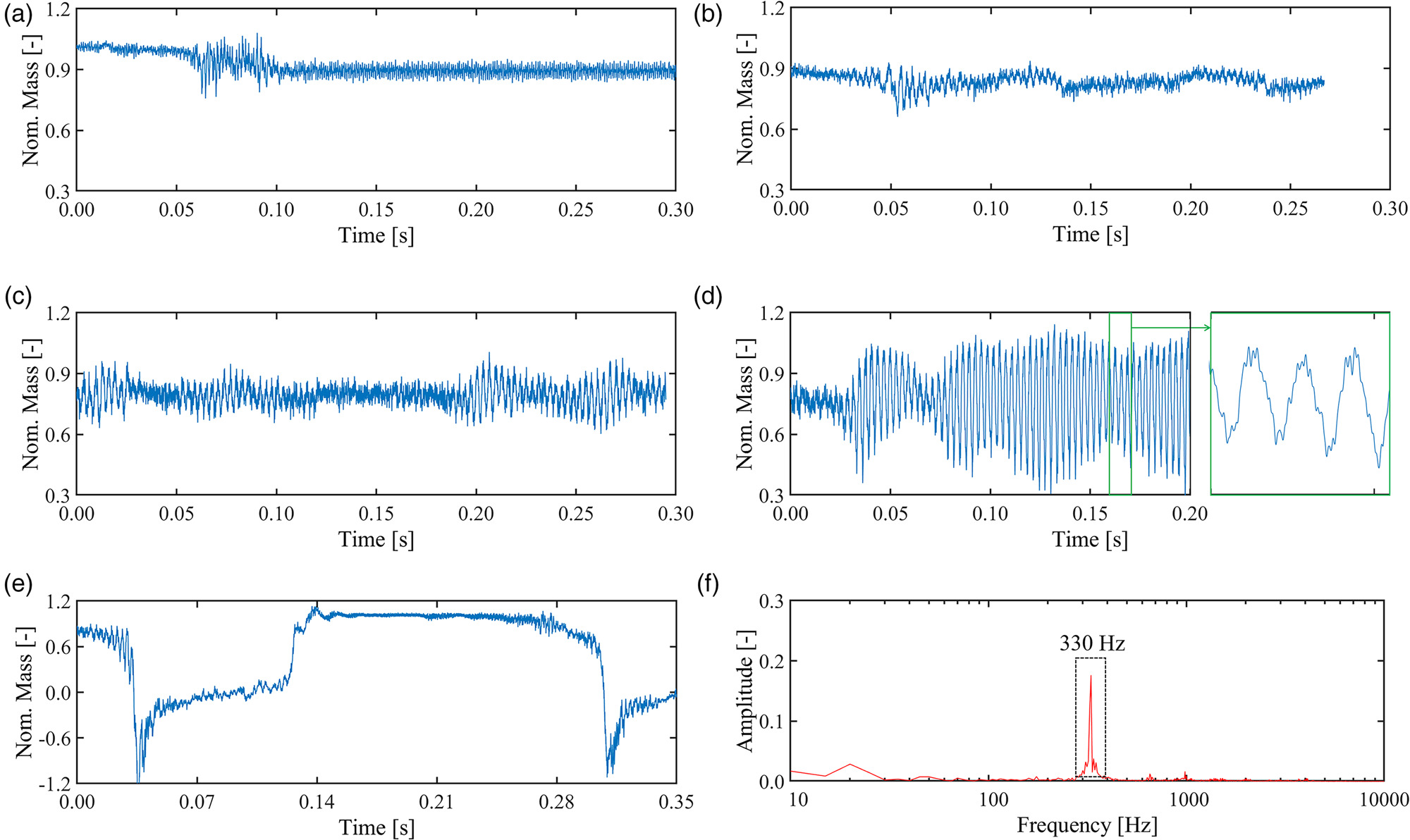
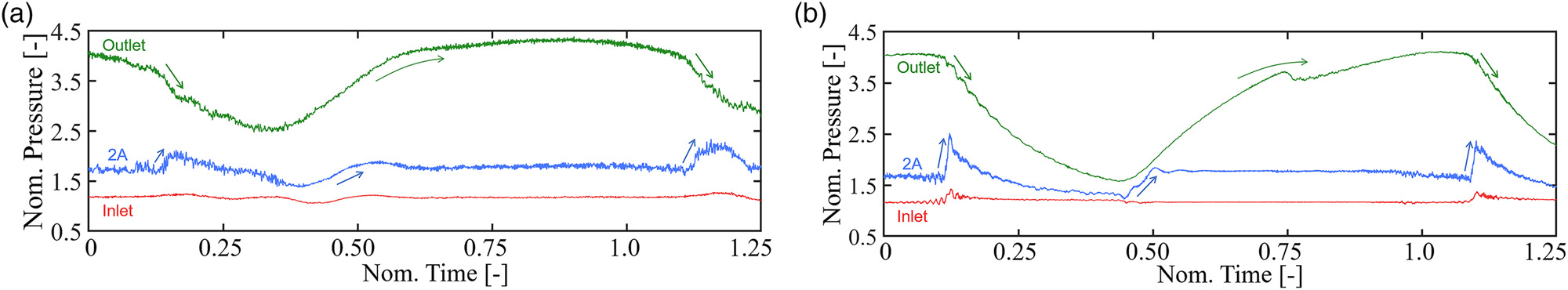
Figure 6 compares the pressure history of a deep cycle in CFD and the experiment at the compressor inlet, 2A outlet, and compressor outlet (marked as Inlet, 2A, and Outlet, respectively). The x-axis is the time normalized by cycle period, and the y-axis is the pressure normalized by the reference value pref (defined by Eq. (7), where ρ is the atmospheric density, and U is the tip velocity at impeller trailing edge). From the perspective of pressure trend, the CFD results agree well with the test data. Therefore, the conclusions drawn from the CFD results are credible.
Two main patterns have occurred from choke to surge at this speed. One is the mild surge, and the other is the deep surge at P5. The following sections will give more details concerning these two phenomena.
Mild surge
This section takes P4 as the focused condition, of which the mass flow rate history has been shown in Figure 5d, and its frequency spectrum is shown in Figure 5f. The frequency of this oscillation is 330 Hz, which is larger than the traditional mild surge. Figure 7 further shows pressure history at different streamwise positions, and the right figure is an enlarged part of three mild surge cycles. The y-axis is the area-averaged static pressure, which is normalized by the time-averaged value. 1A represents the transient characteristic at the outlet of the first axial stage, and so are 2A and 3A. RD denotes the mid-plane between the radial diffuser and axial diffuser.
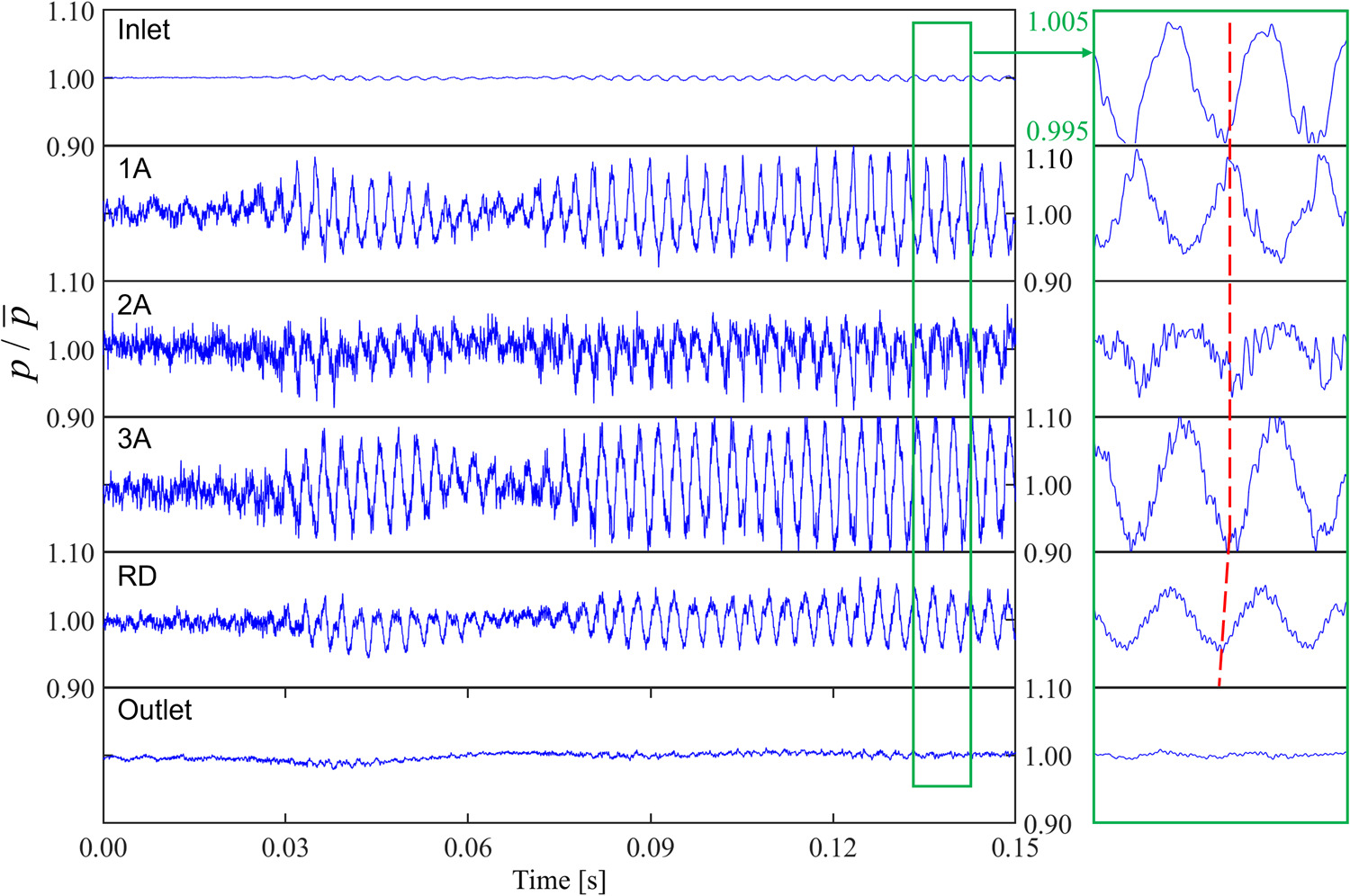
In the right part of Figure 7, a clear anti-phase appears between the inlet and 1A outlet, which is the same case between 1A and 2A. Generally, the transmission of pressure waves is quite fast, almost equal to sound speed. Therefore, the pressure wave causes very little phase difference between streamwise positions, and it is not the pressure transmission that generates an anti-phase in the first and second stages. The front stages are more likely to suffer instabilities for a multi-stage compressor because of the matching between different stages. When the front axial stages work near surge, the latter centrifugal stage works far from the surge boundary. In contrast, the centrifugal stage has stronger workability, which has a stabilizing effect on the front stages. Therefore, when the axial stages entered surge, the centrifugal stage would make them recover to normal conditions. The instability of axial stages causes hysteresis, which explains the anti-phase phenomenon.
Deep surge
As the valve opening decreases, 3A1C enters the deep surge, condition P5, which has a strong reverse flow through the mainstream. The deep surge is usually divided into four phases (Cumpsty, 2004): ① collapse, ② reverse, ③ recovery, and ④ re-pressurization. Figure 8 shows the transient history of inlet mass flow rate and pressure in a deep surge cycle. Condition P5 was initialized by P3, so the amplitude became larger and larger at the first 0.03 s, and finally broke down. The gas stored in the downstream plenum reversed in the following 0.1 s, and when the outlet pressure reached Nom. Pressure = 1.5, the airflow went forward again, which meant 3A1C recovered its workability. Then, 3A1C worked stably until the next surge was initiated.
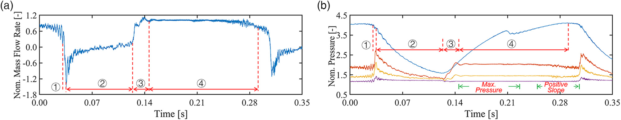
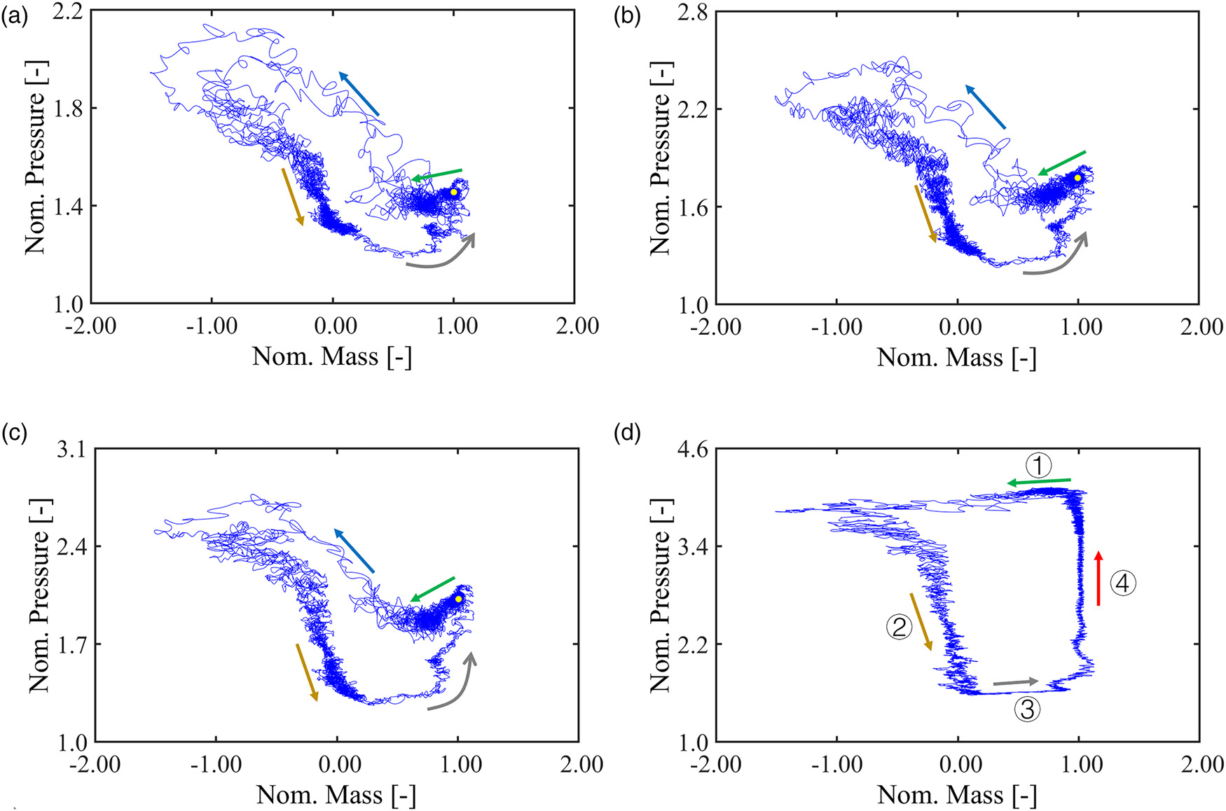
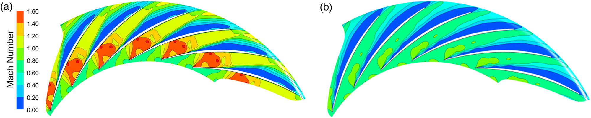
The surge cycles of each stage are shown in Figure 9, where the x-axis is the normalized mass flow rate, and the y-axis is the normalized pressure at different planes. For the axial stages, when 3A1C works near surge, the slope of the characteristic line has changed from negative to positive, as shown by the green arrows in Figures 9a–9c. After the collapse, the pressure at each plane became higher (the blue arrows) because of the reversed high-pressure air. Usually, the positive slope of the characteristic line denotes bad flow conditions, where the compressor can easily evolve into aerodynamic instabilities such as surge. Figure 9d shows the surge cycle at the compressor outlet, and it has a little positive slope before the surge, though the characteristic lines of the three axial stages are steeper. This further shows that the centrifugal stage works stably when the axial stages work near surge. The reverse period, which is a quasi-steady process, can represent the characteristics of axial stages in the negative mass flow rate range. The next process, recovery, is also quite fast. In this process, the operating point of each axial stage moved from the zero-flow point to the peak pressure point, as shown by the grey arrows and yellow points. At the initial moment of re-pressurization, 3A1C worked at the deep choked condition, and a shock wave appeared in the vaned diffuser passage, limiting the mass flow rate. The shock wave (shown in Figure 10a) stops the information transmission from downstream to upstream, so the pressure at the outlet of axial stages keeps almost constant from 0.14 to 0.21 s (Figure 8b). In contrast, the pressure at the compressor outlet increased gradually. When the Nom. Pressure increased to 3.5, the shock wave became weaker and disappeared (Figure 10b), and downstream high-pressure air moved the operating points of axial stages to the characteristics with positive slope gradually, then the next surge cycle happened.
Aerodynamic loads
The final result of aerodynamic instabilities is the structure failure. The sudden crush of high-pressure air could destroy the adjustable housing. In past experiments, these structures and some transducers, such as angular displacement sensors, are more prone to be damaged. In this paper, the IGV, the first and the second axial stators of 3A1C are adjustable. Therefore, it is necessary to evaluate the aerodynamic forces during surge.
Figure 11 shows the history of aerodynamic loads during surge, of which y-axis is the axial force of the rotor blade surface, normalized by the value at the stable condition. For the axial rotor, the negative value denotes reversed pressure gradient. In Figure 11a, the amplitude of R1 force is the largest among three axial stages and reaches 8 times the initial value. Moreover, the axial force changes its direction during the reverse stage ② and keeps positive until the recovery stage happens. Finally, all stages recovered to the normal value in the re-pressurization stage. 1st axial rotor suffers the most violent aerodynamic loads during surge. Apart from the rotor, the axial aerodynamic force of stator is also shown in Figures 11c and 11d, and the IGV has a larger amplitude than other stator rows. Therefore, the front blade rows are prone to have the largest unsteady aerodynamic force.
Figure 11.
Axial Aerodynamic Force on Blade Surface During Surge. (a) R1, R2 & R3, (b) Impeller, (c) IGV, (d) S1 & S2.
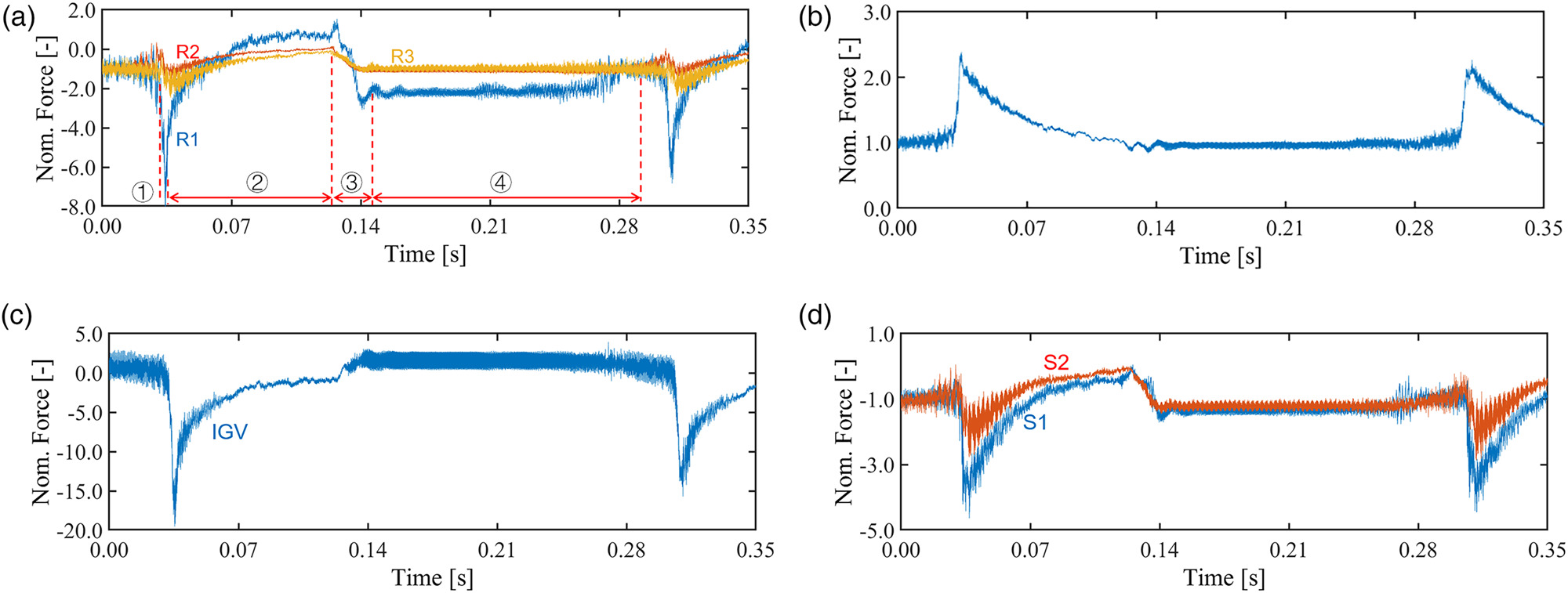
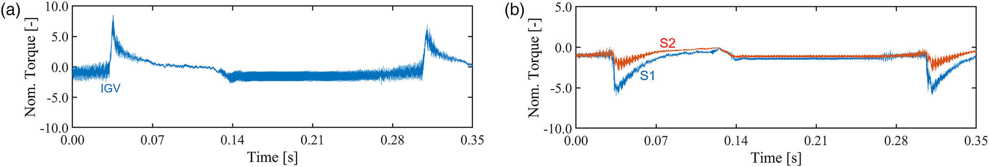
Figure 12 is the torque history of IGV, S1, and S2, of which the y-axis is also normalized by the torque at the stable condition. The trend of torque history has similar conclusions as that of force. The front inlet guide vanes suffer the most violent torque crush, and the direction also changes in the collapse stage. The axial stators of the first and second stage have smaller torque oscillations, as shown in Figure 12b. The pre-tightening torque of the adjustable structure should remain in a reasonable range. The low limit should be higher than the largest aerodynamic torque in the whole experiment to ensure the fixed position of the blade stagger, and the up limit should be lower than the largest torque of the driven motor. Therefore, torque evaluation is necessary before the experiment.
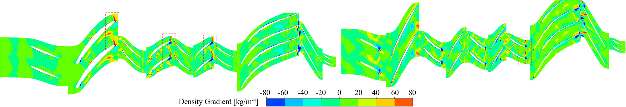
Apart from the axial aerodynamic force and the torque of adjustable stators, some reverse flow also can damage the blade structure. According to Schoenenborn and Breuer’s (2012) research, a shock wave caused by reverse flow would appear at the impeller trailing edge, leading to some cracks. This paper also investigated the flow field based on CFD results. Figure 13 shows the density gradient contour at t = 0.035 s when the negative mass flow rate reaches the maximum. The left figure is the density gradient contour at 10% span, and the right shows the contour at 90% span. As shown by the dotted box in the figures, the shock wave caused by reverse flow appears at lower spanwise positions of the rotor trailing edge and higher positions of the stator trailing edge. Different spanwise positions should be focused on when designing the structure.
Conclusions
This paper investigates a 3A1C combined compressor at the off-design speed, and its instability process is carefully investigated based on the CFD model. The conclusions are drawn as follows.
The compressor studied in this paper suffers a high-frequency mild surge, which has a higher order than that of the traditional mild surge. In addition, the transient pressure history shows an anti-phase between the inlet, 1st stage outlet, and 2nd stage outlet. It is considered that the stabilizing effect of the centrifugal stage leads to such a high-frequency oscillation.
The flow behaviour of each stage is investigated in the deep surge cycle. At the recovery stage, the operating points of axial stages move from the zero-flow point to the peak pressure point directly instead of moving along the steady performance curve. This is mainly because the radial diffuser is choked, limiting the mass flow rate.
The aerodynamic loads during deep surge are evaluated. The results show that the front blade rows have the largest oscillation amplitude, in which the unsteady force of IGV had reached 20 times larger than the normal steady value. Therefore, the transient torque on adjustable stators is necessary to be calculated before the experiment because the stagger may be changed if pre-tightening is insufficient for the regulating equipment of variable stator vanes.
The numerical result of the flow field shows that the rotor's low spanwise part and the stator's high spanwise part are prone to suffer flow impulse shock during surge cycle, and such positions should be focused on in the design of structural strength.
Nomenclature
p
Pressure
ρ
Atmospheric Density
U
Tip Velocity
1D
One-Dimensional
3D
Three-Dimensional
1A
First Axial Stage
2A
Second Axial Stage
3A
Third Axial Stage
R1
First Axial Rotor
R2
Second Axial Rotor
R3
Third Axial Rotor
S1
First Axial Stator
S2
Second Axial Stator
S3
Third Axial Stator
RD
Radial Vaned Diffuser
PR
Pressure Ratio
Nom.
Normalized Parameters
IGV
Inlet Guide Vanes
3A1C
Three-Stage-Axial and One-Stage-Centrifugal Combined Compressor
1D–3D
One-Dimensional–Three-Dimensional Coupled Method