
Introduction
Further increasing the propulsor efficiency and decreasing the environmental impact of aviation is a challenging task, that requires ongoing research of new aircraft and especially propulsion technologies. Currently, there are a couple of promising development trends. On the one hand, fuselage- or wing-embedded propulsors show promising increases in efficiency, according to (Gunn and Hall, 2014) and (Uranga et al., 2017). On the other hand, further increases in the bypass ratio and decrease in fan pressure ratio of UHBR engines are also known to significantly improve the propulsor efficiency (Cumpsty, 2010). While boundary layer ingesting (BLI) propulsors inherently face the problem of asymmetric inlet conditions due to ingested boundary layers, asymmetric inlet conditions are of particular interest in the case of increasing bypass ratios. This is because this development trend requires a necessary reduction in inlet length to compensate for weight and drag losses that arise due to increasing bypass ratios (Peters, 2014). With decreasing fan pressure ratio, the fan becomes more susceptible to perturbations in the flow, thus making a reduction in inlet length even more critical, since flow separation is more likely to occur during operation with high angles of attack, e.g., maximum climb or crosswind conditions (Seddon and Goldsmith, 1985). In both cases, it is important assess the performance of the fan and the components downstream under off design conditions as early as possible in a design cycle. However, full-annulus CFD simulations are necessary to capture the highly inhomogeneous flow that occurs during these off design conditions. However, such simulations require large amounts of computer resources, which is limiting during the early design phases. Reduced Order Models are a useful resource to consider the coupling between engine inlet and fan during the early design phases. In this paper the body force modeling (BFM) method will be assessed. This model uses source terms added to the Navier Stokes equations to represent the aerodynamic behavior of the blades in a circumferentially averaged manner without having to consider the blades spatially discretized, which significantly reduces the mesh size. This approach enables the steady simulation of a full- annulus fan stage within an intake under distorted inflow conditions - e.g. due to high angle of attack or crosswind - with drastically reduced computational cost.
First introduced by Marble (1964), the BFM approach was used in several studies. For example Gong et al. (1999) used the BFM approach for stall inception and distortion transfer, which was later used by Hsiao et al. (2001) to investigate the rotor’s effect on inlet flow separation in a powered nacelle. Another field of application is the simulation of fan noise, which was done by Defoe et al. (2010). Peters (2014) used a modified version of Gong’s model to build a design framework for ultra short nacelles for low fan pressure ratio propulsors. More recently Hall et al. (2017) proposed a new model formulation that eliminates the a priori calibration process necessary in earlier BFM applications making it even more suitable during early design phases. They validated the model’s capabilities with experimental data by Gunn and Hall (2014). However, their proposed model did not include a loss model, but a diffusion factor to consider efficiency. This model has been modified by Thollet (2017) in order to make it viable for the application on transonic fan stages with a newly proposed loss model and metal blockage consideration. The main goal of the present paper is to evaluate a body force model, that is capable of resolving the aerodynamics of transonic fan stages. Therefore, the model by Thollet (2017) will be applied to a transoinc fan stage and its results will be compared to conventional single passage simulations.
Methodology
The body force modeling approach replaces a physical blade row with an empty volume, in which a body force field is used to simulate the effects of the physical blades on the flow. This approach models the equivalent of the pitchwise averaged blade aerodynamics, as shown in Figure 1.
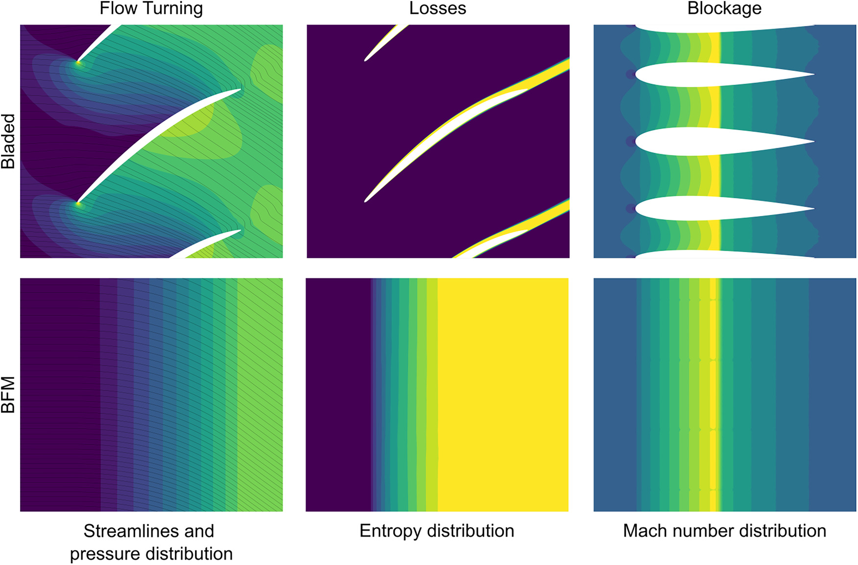
While the approach is capable of producing similar flow turning and pressure rise, it does not capture local phenomena such as loss wakes, as can be seen in the contours of entropy. The modeling approach must account for the geometrical blockage caused by a physical blade row, as evident in the contours of Mach number in Figure 1.
The local body force f is calculated based on Equation (1),
where
Figure 2.
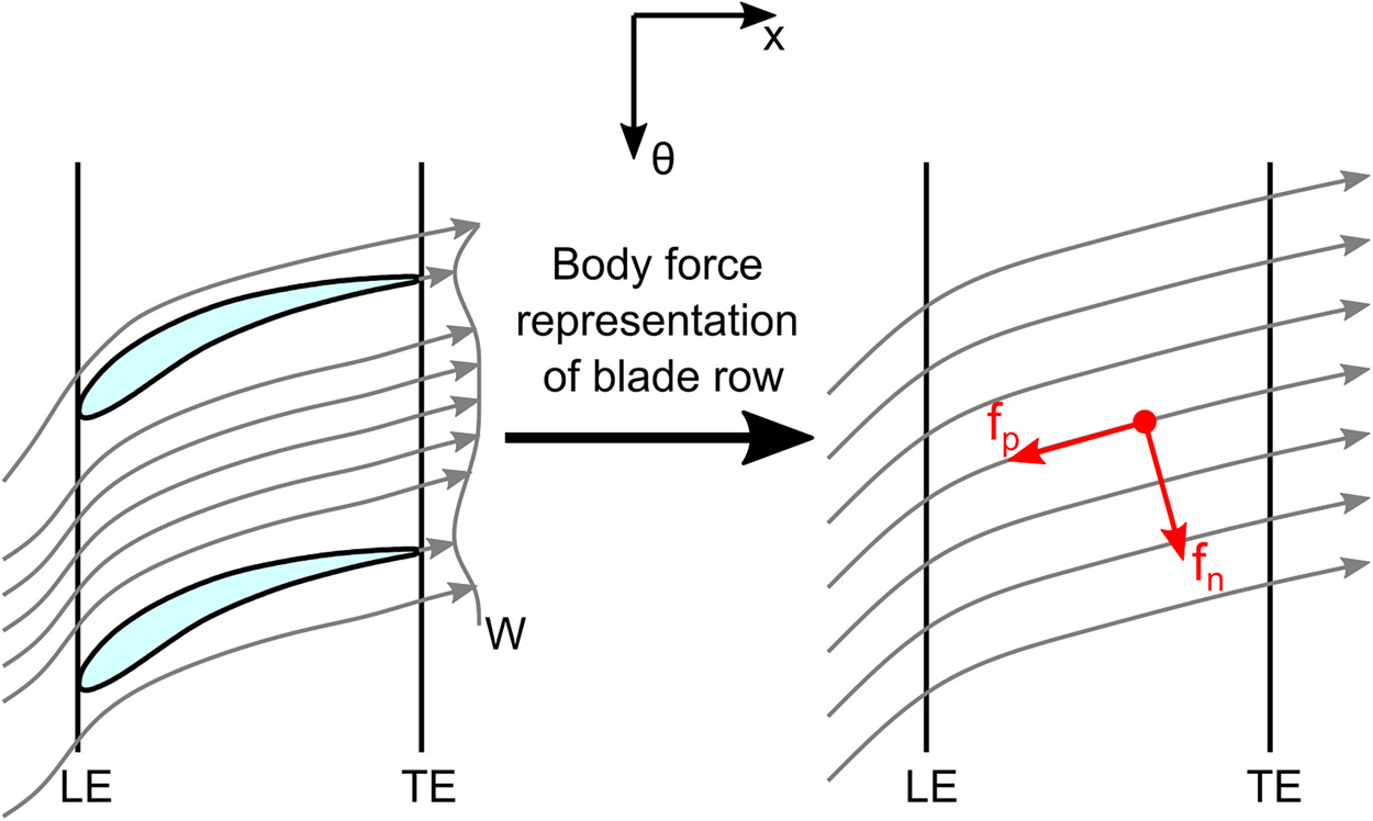
Relative flow through discrete blade passage (left) and relative flow through body force field (right). (Peters, 2014).
Governing equations
The governing equations for the body force approach are those for mass (2), momentum (3) and energy conversation (4), (Liepmann, 2013):
In the momentum equation the body force f gets added within the term
Numerical setup
Due to the nature of the body force model, there is no circumferential variation in the model equations. The blade row gets modeled in an axisymmetric way. A comparison of the numerical setups of a bladed simulation versus a body force simulation is pictured in Figure 3.
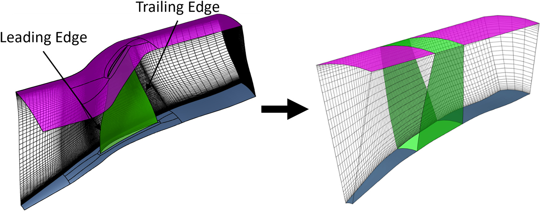
Figure 3 illustrates a key advantage of the body force approach over traditional bladed domain simulations. In the bladed domain, it is necessary to have a high spatial discretization of boundary layers. On the other hand, the BFM domain can be spatially resolved much more coarsely, since there is no need to resolve the blade boundary layer. To create the mesh for the BFM domain, a 2D mesh is created in the meridional plane and then rotated in the circumferential direction, thus adding cells in the circumferential direction. This requires only information about the endwall geometry, as well as the location of the leading and trailing edge.
Unlike the axisymmetric nature of the BFM setup, the model can react locally to non-axisymmetric inflows. Therefore, the model is able to accurately simulate the effects due to inflow disturbances.
State of the art
The calculation of the two body force components
Hall’s model uses the blade camber surface geometry as a priori input and can be expressed as follows:
The local inviscid body force is determined by equating the local deviation angle
Although this model was capable of predicting the inviscid redistribution effect of a BLI propulsor, it could not predict efficiency, as Hall neglected the
Further improvements were made by Thollet (2017) by
Loss model
The main limitation of Hall’s model was its inability to capture losses. Thollet uses a simple formulation which relies on the local friction coefficient
This leads to the loss fomulation:
The off-design term in Equation (8) is determined using the distribution of the deviation angle
Blockage effects
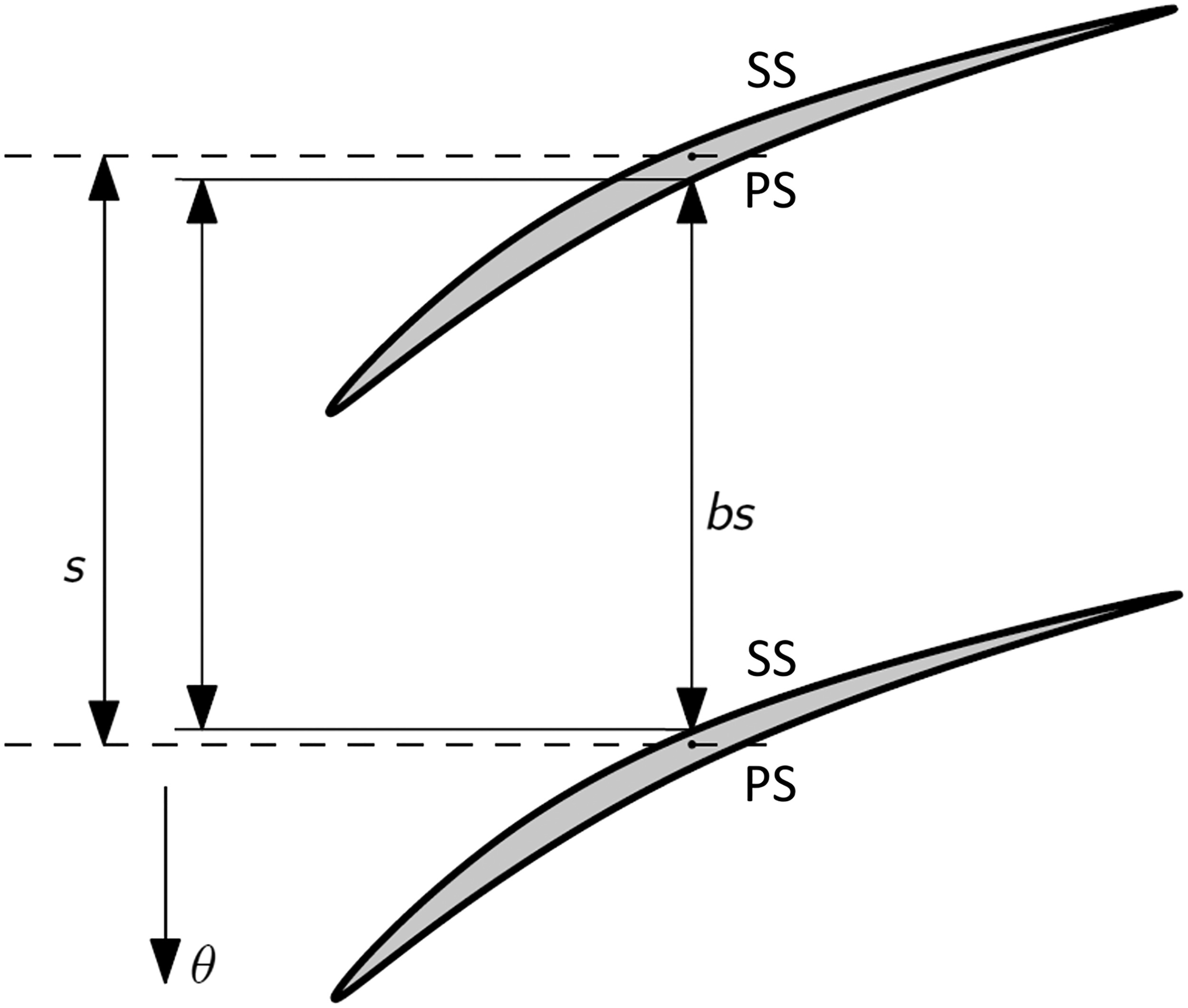
In order to account for metal blockage effects and its influence on the choking mass flow, based on the reduction in effective flow area due to the presence of physical blades this has to be modeled within the body force approach. Therefore, a blockage factor b is introduced. The blockage factor b is a dimensionless factor that equates the camber to camber pitch distance s of two neighboring blades to the geometrical distance between pressure and suction side of these two blades. This parameter accounts for the reduction of effective area within a blade passage, as pictured in Figure 4.
It is calculated by
The blockage factor is included within the governing Equations (2)–(4):
Compressibility correction
The original model by Hall was tested on incompressible test cases. Thollet has proven, that the following correction yields a valuable impact for transonic configurations. The baseline model of Hall is based on the lift coefficient of a thin airfoil at low Mach numbers, but the lift coefficient of an airfoil increases at high subsonic Mach numbers and has a different expression for supersonic flows. Therefore, a compressibility correction is added
which is an derivation of the Prandtl-Glauert correction for subsonic mach numbers and of the Ackeret formula for supersonic mach numbers. In order to avoid the singularity near
Resulting equations
These modifications lead to the following model formulation for the inviscid and viscous body forces (Thollet, 2017):
The necessary input for the model is the distribution of the metal angle
Implementation in solver
The results presented in this paper were obtained through the use of ANSYS CFX 21R2. ANSYS CFX uses a coupled solver, which solves the hydrodynamic equations as a single system with a fully implicit discretization of the equations (ANSYS Inc, 2021). In order to use the body force approach in CFX, it is necessary to divide the domain into several subdomains. The subdomains representing the rotor and stator have additional sources corresponding to
Local blockage can be modeled, by defining a local volume porosity
Results and discussion
First, we discuss the blockage model and its performance in comparison to bladed simulations. Next, we evaluate the model’s ability to predict compressor aerodynamics by using a transonic fan stage test case.
Blockage model
The blockage model was tested using a generic NACA0016 geometry (Eastman et al., 1933) as a stator. Since the geometry is a zero lift profile, there are no resulting inviscid body forces
Figure 5.
Stator test case. (a) Numerical setup of NACA0016 stator test case. (b) Blockage Factor distribution of NACA0016.
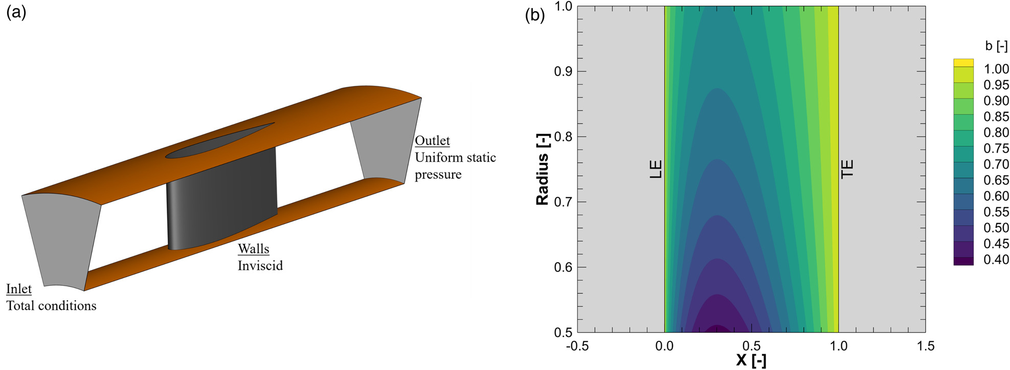
The distribution in Figure 5(b) shows the geometric relationships for the blockage factor. Towards the leading and trailing edge the values of blockage factor approach
Figure 6.
Contour plots of the Mach number at midspan for the NACA0016 stator test case. Subsonic conditions (left) and transsonic conditions (right). (a) Bladed Simulation with subsonic conditions. (b) Bladed Simulation with transsonic conditions. (c) BFM with subsonic conditions. (d) BFM with transsonic conditions.
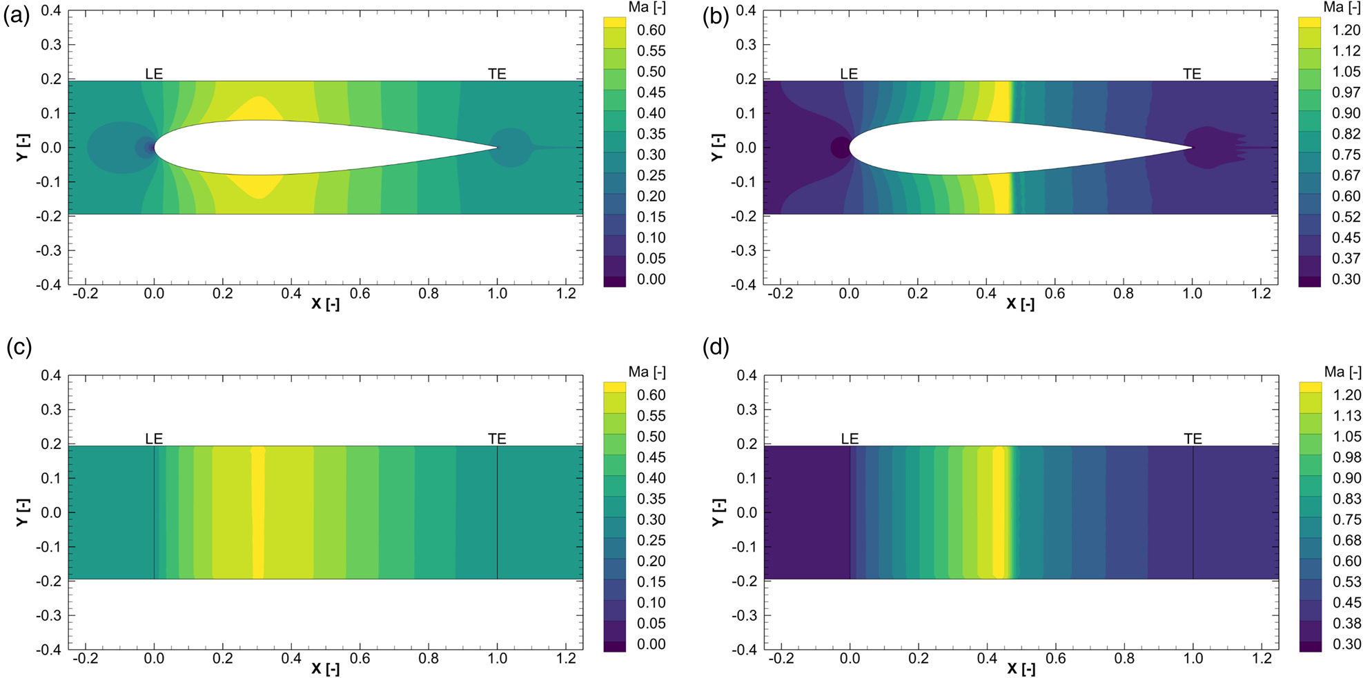
Figure 7.
Circumferentially averaged Mach number at midspan from inlet to outlet for the NACA0016 stator test case. Subsonic conditions (left) and transsonic conditions (right). (a) BFM vs. Bladed Simulation with subsonic conditions. (b) BFM vs. Bladed Simulation with transsonic conditions.
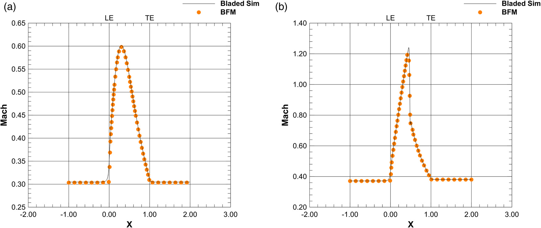
Figures 6(a) and 6(c) illustrate the Mach number distribution for subsonic flow conditions. The axisymmetric nature of the body force model is evident in Figure 6(c), where no gradients in the Y direction are present. Both models accurately capture the flow acceleration in accordance with the Bernoulli equation, as demonstrated in Figure 7(a), where the circumferential averaged Mach number at midspan from inlet to outlet is compared. The BFM approach is capable of reproducing the magnitude, location, and slope of the Mach number peak, except for the onset of acceleration at the leading edge, which is not perfectly captured due to the missing stagnation point and its effect on the upstream flow in the BFM approach.
For transonic flow conditions, Figures 6(b), 6(d), and 7(b) depict the Mach number distribution. Similarly, the BFM approach accurately predicts the flow behavior, including the position of the shock and the faster flow downstream of the stator. However, the strength of the shock is underestimated, and the onset of acceleration at the leading edge of the stator is slightly underestimated as well.
These results demonstrate that the BFM approach, developed from Equations (10)–(12), can effectively capture metal blockage effects for the inviscid case. However, it should be noted that the validation of metal blockage has only been conducted for the inviscid case. For boundary layers due to viscous walls, the effective area between two neighboring blades decreases even more, which increases blockage due to aerodynamic effects. This aspect has not been addressed in this study but is left for future investigations. In addition, a relatively straightforward calculation was utilized to determine the blockage factor b. In previous studies, Baralon (2000) proposed an alternative approach to compute the blockage factor b. Unlike the approach adopted here, Baralon calculates the blockage factor perpendicular to the camber surface. Notably, Baralon was able to achieve encouraging results with the NASA 67 rotor. This approach is planned to be investigated further in future work.
Transsonic fan stage
In the following, the model is tested using a transonic fan stage. For this test case the CA3ViAR (Composite fan Aerodynamic, Aeroelastic, and Aeroacoustic Validation Rig) fan stage is used (Eggers et al., 2021) which features a composite low-transonic fan. Its fan stage characteristics are shown in Table 1.
Table 1.
CA3ViAR fan stage characteristics.
To evaluate the accuracy of the model, a bladed simulation is conducted in conjunction with the BFM simulation. The numerical configurations for both simulations are displayed in Figure 8(b), with identical boundary conditions applied. The inlet is subjected to total conditions, while the outlet is maintained at a static pressure with radial equilibrium. With the exception of the horizontal hub in front of the spinner, all walls are assigned as viscous walls. For turbulence closure, the
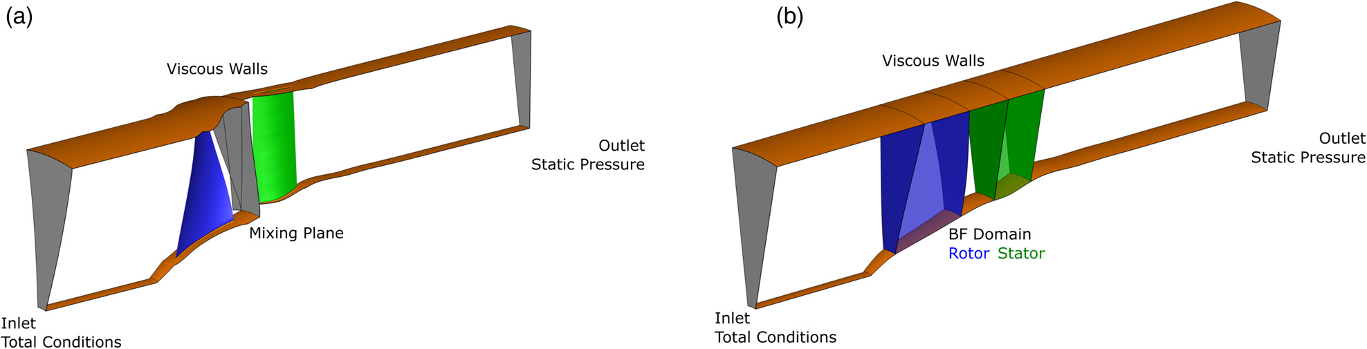
Table 2.
Mesh Stastistics for the CA3ViAR Setup.
| Mesh | Bladed Sim. | BFM |
|---|---|---|
| No. of Elements | 3.747.456 | 1.039.300 |
| Domain Size | 1 Passage (1/18 Rotor and 1/40 Stator) | 20° segment |
Figure 9 compares the results of bladed simulations and the body force approach for the Cruise and T/O operating points listed in Table 1. Speedlines were calculated for each operating point, and the total pressure rise over the fan
Figure 9.
Compressor Map for the CA3ViAR fan stage test case, pressure ratio π t , Fan η poly
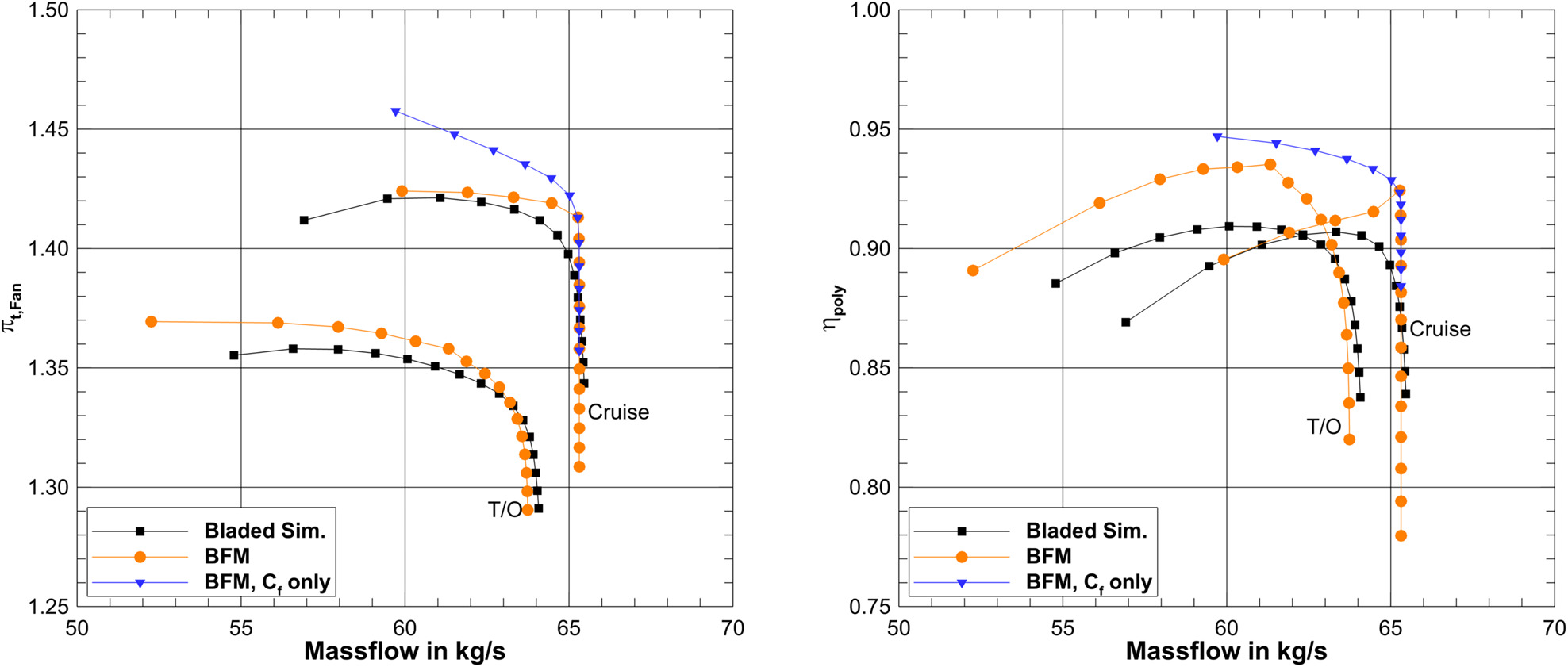
The results demonstrate that the BFM approach accurately predicts the choke mass flow for both operating points. However, at lower mass flow rates, the BFM approach slightly overestimates the total pressure rise. The impact of the off-design term from Equation (8) can be observed by comparing the blue line to the orange line, which shows that the design term causes the slope of the speedline to decrease from the point of maximum efficiency towards lower mass flows. Without this term, the efficiency and work of the fan would be overpredicted by the BFM approach. However, even with the off-design term, Figure 9 shows that the efficiency is overpredicted by approximately
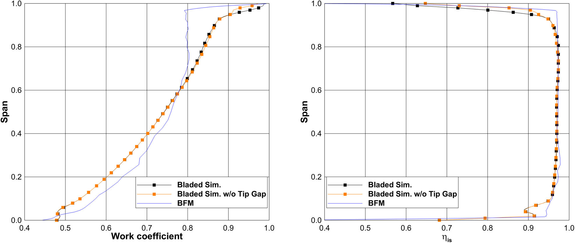
Figure 10 presents the local result quality of the BFM approach, where the spanwise distributions of the work coefficient and isentropic efficiency downstream of the rotor are shown in Figure 10. These figures demonstrate that the BFM approach provides satisfactory results for the maximum efficiency operating point at the T/O operating condition. However, discrepancies in the model are evident in predicting the work input of the rotor accurately. The BFM overestimates the work input close to the hub and underestimates it in the direction towards the shroud, which is consistent with the findings in (Thollet, 2017). The lack of consideration of the tip gap does not justify this deviation. To further investigate this, a bladed simulation without a physical tip gap was performed, and the results are shown in the orange line. As expected, the absence of the peak gap increases the work input close to the shroud compared to the bladed simulation with a tip gap. However, this does not explain the spanwise distribution of the BFM approach. The isentropic efficiency in Figure 10 also shows similar behavior, where the BFM approach overestimates the isentropic efficiency near the hub and shroud but agrees precisely with the results in the core region of the flow.
Conclusions
In this study, a state-of-the-art body force model is considered to evaluate its ability to predict the aerodynamics of a transonic fan. To assess the model’s performance, the basic model was used along with modifications from the literature, and its blockage modeling functionality was validated using a simple stator test case. Following this, the model was applied to the CA3ViAR fan stage, where satisfactory results are obtained with one third of the mesh size compared to a bladed simulation. However, limitations of the model were also identified, which were previously documented in the literature.
Despite these shortcomings, the model serves as a valuable starting point for future modifications to improve its performance, particularly with respect to the tip gap aerodynamic. Previous works (Xie and Uranga, 2020, 2021), have attempted to modify the model, but the results are found to be insufficient for the transonic fan presented in this study. Thus, future research will focus on developing and testing new modifications to the model to address these limitations.
To validate the model, accompanying experiments will be performed using the INFRa rig (Grubert et al., 2022) at the Institute of Jet Propulsion and Turbomachinery. These experiments will not only investigate fan aerodynamics but also inlet distortion, which will be further studied in future work using the body force model. Overall, this study provides valuable insights into the capabilities and limitations of the body force model and highlights directions for future research.
Nomenclature
Latin
Blockage factor (−)
Local friction coefficient (−)
Body force per unit mass (m/s2)
Enthalpy (J)
Compressibility correction factor (−)
Mach number (−)
Number of blades (−)
Surface normal (−)
Pressure (Pa)
Radius (m)
Local Reynolds number (−)
Pitch (m]
Momentum source (kg/m2s2)
Energy source (W/m3)
Time (s)
Physical Volume (m3)
Virtual Volume (m3)
Velocity (m/s)
Cartesian coordinates (m)
Abbreviations
BFM
Body Force Model
BLI
Boundary Layer Ingestion
LE
Leading Edge
NACA
National Advisory Committee for Aeronautics
NASA
National Aeronautics and Space Administration
MFR
Mass Flow Rate
PTF
Propulsion Test Facility
PS
Pressure Side
RANS
Reynolds Averaged-Navier Stokes
SS
Suction Side
TE
Trailing Edge
UHBR
Ultra High Bypass Ratio