Introduction

Ultra-high bypass ratio (UHBPR) turbofans offer significant reductions in fuel burn and pollutant emissions due to their higher propulsive efficiency. Drag and weight penalties incurred by the associated larger installation diameters can be offset by using short intakes (Hoheisel, 1997). However, shorter intakes lead to stronger fan-intake interaction, which combined with the lower fan pressure ratio could jeopardize the stable operability at off-design conditions. To better understand the off-design behaviour of the fan, and to validate numerical predictive methods, experimental testing is used. The large costs and time-scales of matching the very high Reynolds numbers of engine-scale fan stages make these programmes prohibitive for detailed experimental testing, with further difficulty in accurately instrumenting test facilities. Subscale experimental testing – recreating operational Mach numbers at reduced Reynolds numbers with scaled geometry – presents an affordable and practical route to measuring fan-intake interaction and design changes.

A challenge in producing representative behaviour at reduced Reynolds numbers is the presence of laminar boundary layers approaching the shock wave. This might lead to laminar/transitional shock wave-boundary layer interactions (SWBLIs), which generally do not occur on full-scale transonic fan rotors. An in depth analysis of this type of interaction, including unsteady effects, can be found in Hergt et al. (2019). Briefly, this type of interaction can be characterised by three different types of structures depending on the strength of the shock wave. For a weak shock, the interaction does not separate the boundary layer; instead transition is induced and the boundary layer is thickened. An increase in shock strength leads to induced transition and a separation bubble under the shock foot. For a strong shock, the interaction generates an open boundary layer separation that does not reattach before the trailing edge. For transonic compressor cascades Szwaba et al. (2019) and Klinner et al. (2019) studied laminar SWBLIs on modern compressor blade sections at moderate shock strengths. This type of interaction is characterised by a double shock structure. The upstream weak oblique shock promotes the transition of the boundary layer to turbulent, also inducing separation of the boundary layer. The main shock encounters this separated turbulent region and performs most of the deceleration across the shock. The separation bubble closes behind the shock. The authors found that promoting transition upstream of the shock resulted in a single shock structure with a shorter separation bubble. Due to the difficulties of measuring SWBLIs in a 3D rotating blade row at representative Reynolds number, experimental data is not publicly available. However, allowing laminar boundary layers to interact with shocks in subscale tests presents significant risk of behaviour unrepresentative of engine-scale conditions.

To reduce the risk of a low Reynolds number experimental rotating fan rig, this paper proposes the use of an inexpensive and robust flow control method for the suction side of the fan blade. Design guidelines are given for the location and height of the discrete roughness elements used to control the boundary layer state. This paper also presents a rapid experimental validation methodology to ensure and de-risk the application of the boundary layer trip to the 3D rig blade. The proposed experimental validation enables the rapid investigation of the loading and boundary layer state on the suction side of the fan blade within a variable-density wind tunnel at different span sections, working lines, Reynolds numbers, Mach numbers, surface roughness and boundary layer trip characteristics. The methodology and experimental setup are designed to maximise the control over the experiment, minimise the sources of uncertainty, increase the pace of experimental testing and maximise the range of geometries and operating conditions tested within a modest variable-density wind tunnel. The experimental methodology is applied to a generic aerofoil representative of a fan tip section. The experimental method proves that it is possible to reproduce boundary layers and pressure distributions of a full-scale fan blade on a 1/10 subscale model. The results obtained confirm that the boundary layer trip method successfully promotes transition at the location representative of full-scale blades, avoiding unrepresentative laminar shock boundary layer interactions. This highlights the importance of conditioning boundary layers in low Reynolds number fan rig testing. The boundary layer conditioning is attained with a minimal surface modification, which is readily applicable to existing test models.

Methodology

This sections presents an overview of the collection of numerical and experimental methods used in this study. In the first place, low order models are used to estimate the boundary layer state and possible separation location at different span sections and operating points of the full-scale and subscale rotating rig. In the second place, a boundary layer trip is designed for the subscale 3D blade able to replicate the full-scale behaviour at different operating points. In the third place, symmetric isolated aerofoils are inverse designed to produce representative suction side loadings in an experimental free-jet section. These maximise flexibility and pace of experiment whilst minimising sources of uncertainty and cost. Next, the boundary layer trips designed for the rotating subscale blade are scaled for the experimental isolated symmetric aerofoil and the full details of the experimental techniques are given. The experiments rapidly confirm the boundary layer state of the flow approaching the shock wave and the effectiveness of the flow control.

Computational method

3D Reynolds-averaged Navier-Stokes (RANS) calculations were carried out using Turbostream (Brandvik and Pullan, 2011). For design iterations, boundary layers were modelled as fully turbulent, using the Spalart-Allmaras turbulence model. Flow was allowed to slip at the surface, with wall functions modelling surface shear. Values of y+ less than 2 were used.

A rectangular computational domain was used during the design interations, it provided representative free jet conditions at a very low computational cost. The geometry and boundary conditions of the domains are shown in Figure 1. Uniform total pressure and total temperature axial flow was admitted at the inlet, and uniform static pressure set at the outlet. The boundaries parallel to the free-stream flow applied the same total properties as those at the inlet for flow entering the domain, and the same static pressure as the outlet for flow exiting the domain, with the flow angle taken from the local flow solution. As flow exited the domain upstream of the shock, the fixed static pressure faithfully modelled the effect of the finite jet.

Figure 1.

Computational domain. Flow moves from left to right.

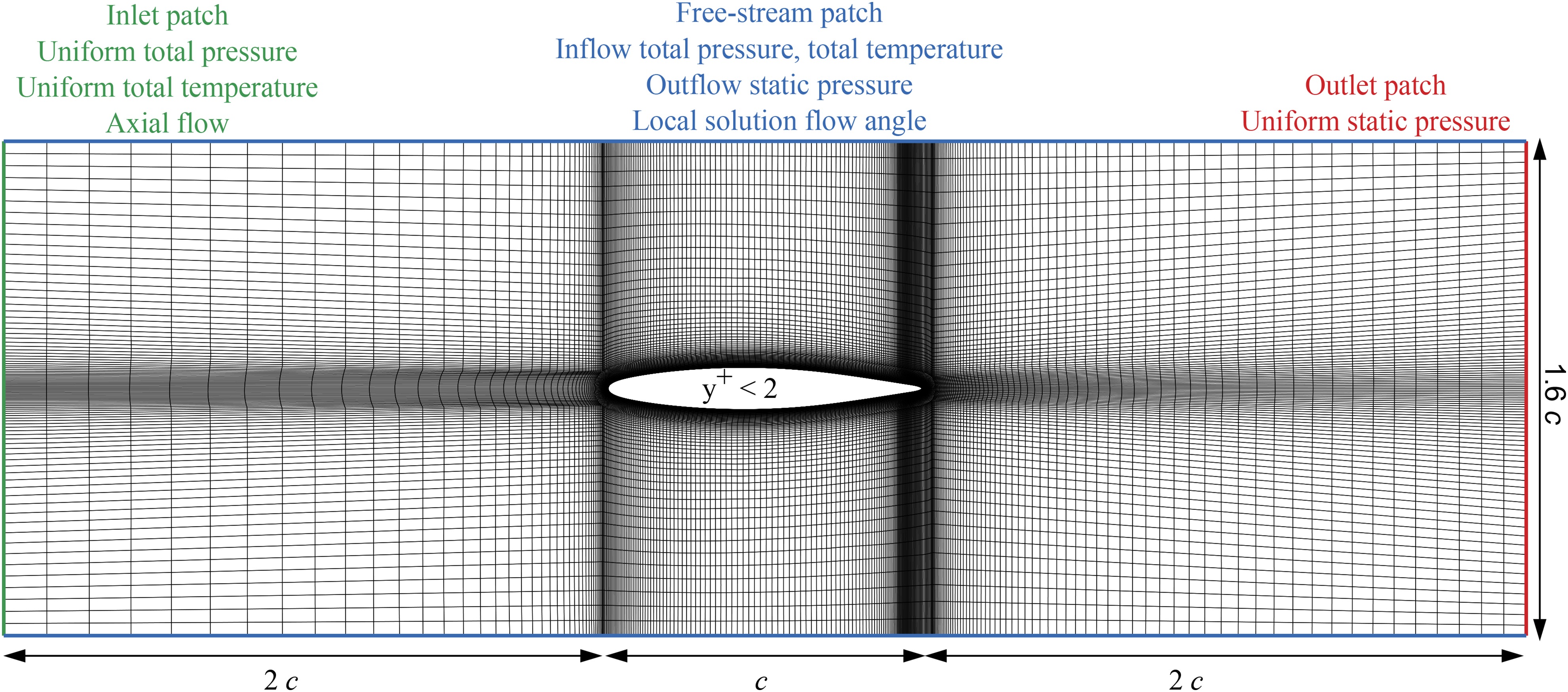
The multi-block, structured grid shown in Figure 1 consisted of around 160,000 nodes. The domains has 5 nodes in the direction normal to the view in Figure 1, with periodic patches connecting the faces in this direction. This maintained 2D flow velocity, representative of a mid-span slice of the rig flow field.

Experimental method

To survey the state of the boundary layer and the shock boundary layer interaction, a new transonic free-jet test section was commissioned and installed within a variable-density wind tunnel at the Whittle Laboratory. This tunnel is a closed loop, continuous running facility which allowed the independent control of the free stream Mach number and aerofoil Reynolds number. All the experiments reported in this paper where carried out at a constant axial Mach number of 0.82 and the density of the working fluid was adjusted to produce chord based Reynolds number ranging from Re=0.54×106 to Re=1.44×106.

Figure 2 depicts the new test section. The section comprised a 3.5:1 contraction nozzle. The aerofoil of interest was immersed in the free jet of the nozzle. The leading edge of the aerofoil was located 0.35 nozzle heights downstream of the nozzle. The flow was discharged into the pressurised wind tunnel. Total pressure was measured far upstream of the contraction. To monitor the free stream Mach number, static pressure measurements within the narrower section of the nozzle were taken using endwall taps. The aerofoils were equipped with 13 0.2mm diameter surface pressure taps located at 25% span, and distributed along the chord to capture the shape of the blade loading. A neptune pressure probe traversed in the pitch direction at an axial location of 50% chord downstream of the trailing edge. The probe measured total pressure, static pressure and yaw angle. All pressure probes/ports were connected via tubing to a 15psi differential pressure transducer. K-type thermocouples were placed upstream of the section to measure the total temperature of the jet. A FLIR A615 infra-red camera, located directly above the aerofoil, measured the steady state aerofoil surface radiosity. The pixel length correspond to 0.25% of the aerofoil chord. An in-house calibration of the camera and the emissivity of the paint applied on the blade was performed. The calibration allowed the estimation of the aerofoil surface temperature based on the radiosity and the tunnel operating conditions. The estimated uncertainties of the main variables of interest are presented in Table 1 for the lowest and highest Reynolds number.

Figure 2.

Free-jet test section. Flow moves from left to right.

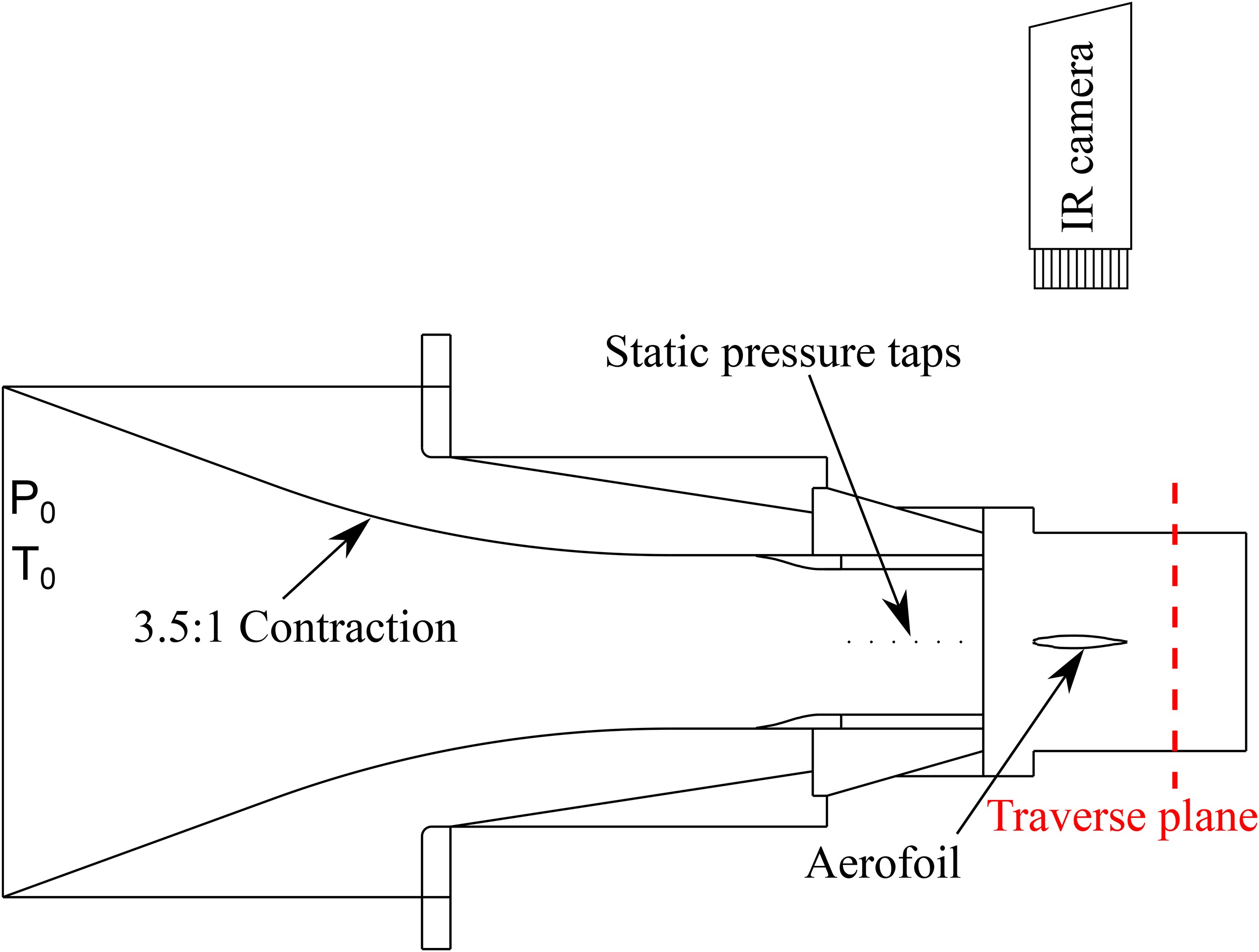
Table 1.

Estimated uncertainties of the experimental data.

	Uncertainty at Re=0.54×106	Uncertainty at Re=1.44×106
Isentropic Mach number (Ms)	±0.002	±0.001
Loss coefficient (Yp)	±0.003	±0.002
Wall temperature (Twall)	±0.2K	±0.2K

During an experiment, pressure and temperature measurements were used to obtain the aerofoil isentropic Mach number distribution and Reynolds number Re. The operating point of the wind tunnel was controlled to match the measured isentropic Mach numbers to the computed fully turbulent isentropic Mach numbers upstream of the shock wave. Additionally, the density of the wind tunnel was changed to precisely control the Reynolds number. For a given roughness height, changing the Reynolds number was effectively equivalent to varying the roughness height for a fixed Reynolds number.

The 2D symmetric sections were manufactured in polycarbonate. This material offers a good compromise between mechanical strength, machinability and thermal conductivity. A target surface roughness Ra=1μm was specified for the manufacturing process. This value was obtained by scaling the rig nominal Ra. The surface of the aerofoil was coated with paint to minimize radiation reflection. Surface roughness measurements of the coated blade were performed with a profilometer to ensure the target Ra was obtained.

The trips designed for the rig were scaled to the symmetric sections. The initial and end position of the trip was scaled geometrically using the procedure previously described. At the location of interest, the design procedure presented above was used to obtain the critical roughness kcrit, boundary layer thickness δ99, and nominal roughness height k. The experimental test could rapidly validate the roughness height bounds of the loss plateau, providing confidence on the design methodology. Spherical microbeads with a tolerance of ±5μm were adhered to the aerofoil surface to build the trip. The same technology can be directly applicable to the rig rotor blades.

The following sections present experimental measurements for a representative generic profile, whose scaled Reynolds number, and aerofoil pre-shock isentropic Mach numbers are similar to those of a fan suction surface tip section. Its geometrical definition is as follows

(1)

(yc)=(xc)12(1−xc)[0.165(1−xc)+0.264xc]+0.007xc.

where an elliptical trailing edge was added in extension to the nominal chord c.

Flowfield with nominal reynolds number - Re = 0.7 × 10⁶

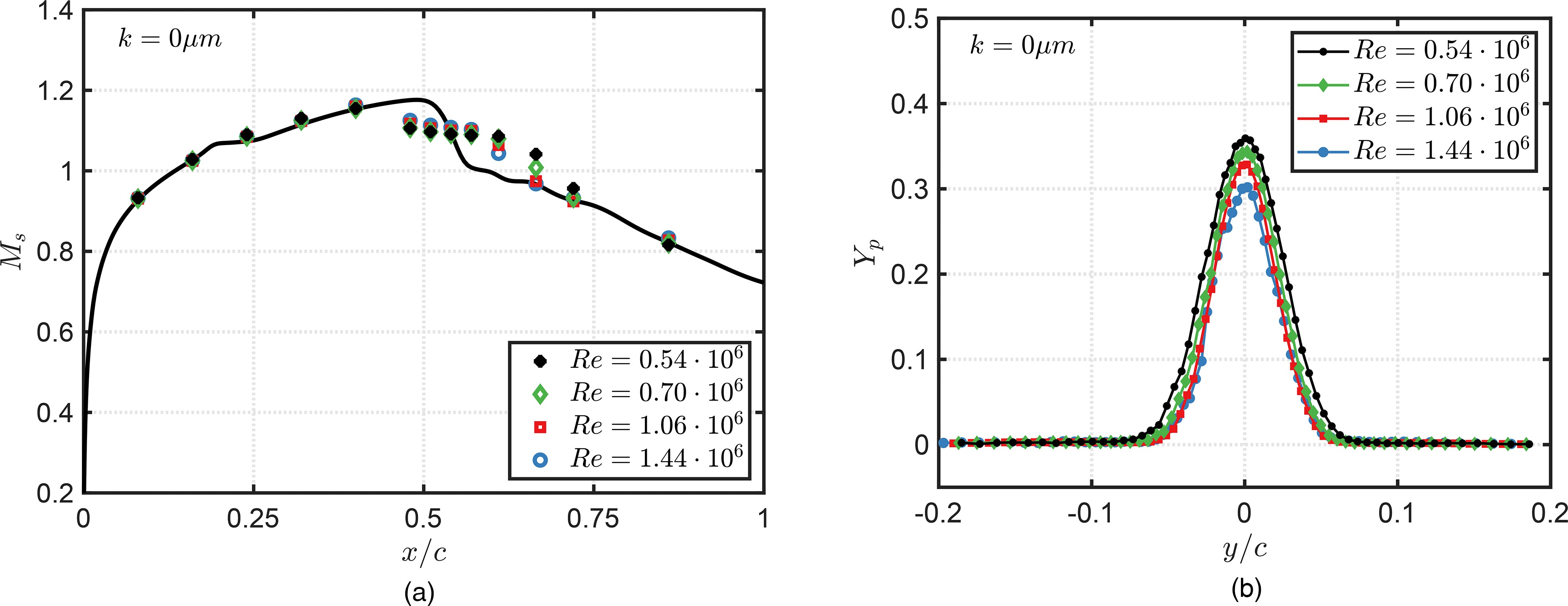
In the first instance, the behaviour of the baseline aerofoil is analysed at the chord base nominal Reynolds number Re=0.7×106. The lower order model does not predict any laminar separation. However, it estimates transition onset at the same location as the shockwave. This case is a representative example of laminar/transitional SWBLIs. Figure 3a presents the experimental isentropic Mach number distributions for the aerofoil without trip (k=0μm) and the nominal trip height (k=82μm) against the design intent distribution, which was calculated using CFD with fixed transition at 18% chord (full-scale Reynods number). For the smooth case (no trip) an early interaction between the boundary layer and the shockwave is observed at x/c≈44%, which leads to an early pressure rise. The pressure rise is followed by a pressure plateau and a second greater pressure rise associated to a late second shockwave. This topology has been previously reported as a transitional SWBLI (Babinsky and Harvey, 2011; Klinner et al., 2019; Szwaba et al., 2019). The adverse pressure gradient imposed by the upstream shockwave separates the laminar boundary layer, resulting in a separation bubble which reattaches at the location of the rear shock. The early interaction induces transition onset, as a result the turbulent boundary layer approaching the second wave is able to withstand a greater pressure rise without causing an open separation. A second CFD prediction is shown in Figure 3a, which was obtained fixing the transition at the location predicted with the low order model for the sub-scale Reynolds number. Excellent agreement is found with the experimental data presented for the smooth case. Tripping the boundary layer with the nominal trip leads to a turbulent SWBLI, which brings the loading distribution back to the design intent. Figure 3b compares the shockwave structure of both CFD predictions. It is shown that the laminar SWBLI leads to a double shock structure, in contrast the turbulent SWBL results in a single shock.

Figure 3.

Effect of baseline trip design on (a) isentropic Mach number, (b) density gradient for Re=0.7×106.

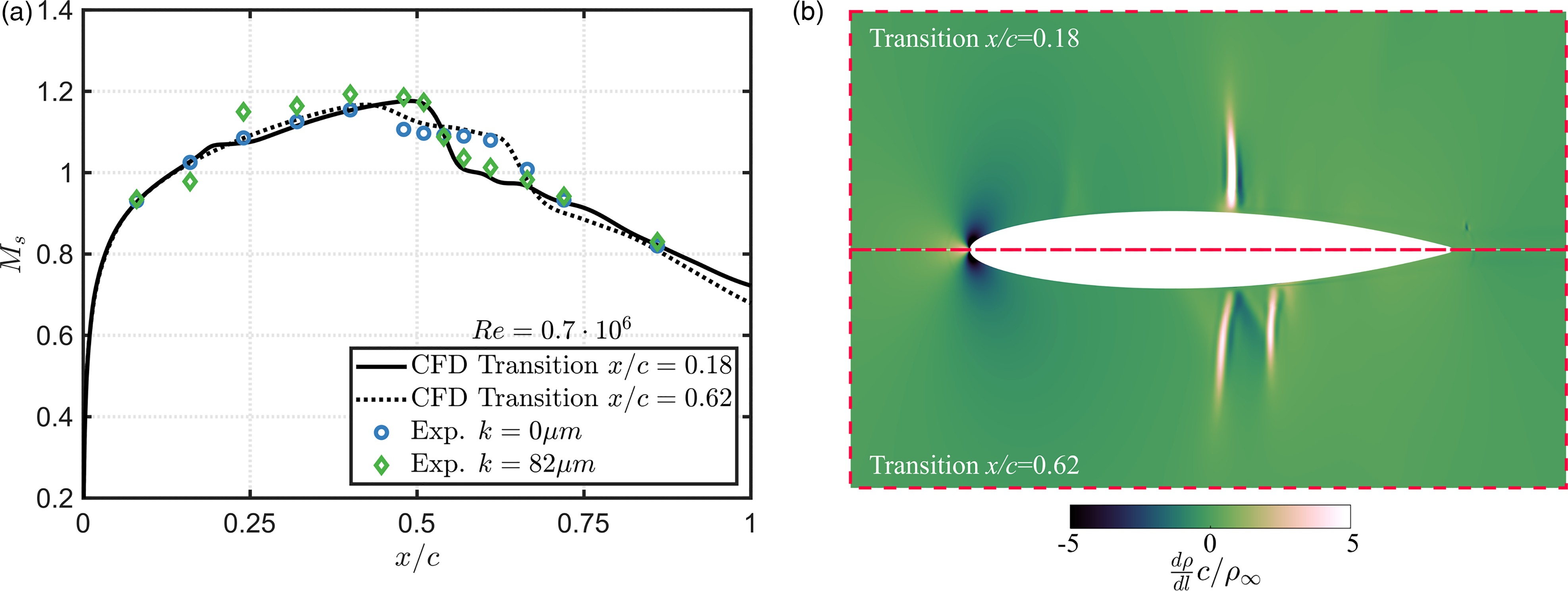
To further investigate the state of the boundary layer, the non-dimensional surface wall temperature field is shown in Figure 4 for both cases. The wall temperature was measured using the infrared camera and it is a function of the free-stream total temperature, local Mach number and boundary layer state. The flow moves from left to right in Figure 4 and the areas upstream and downstream of the blade have been masked in grey for clarity. The locations of the blade pressure taps have been superimposed to relate the loading distribution to the respective wall temperature. As the flow accelerates around the leading edge, the static edge temperature Te drops. In the absence of a boundary layer state, the wall temperature experiences a consistent temperature drop. This is observed upstream of the trip location for both cases. For the nominal trip, the wall temperature rises as the flow crosses the trip. Two scenarios can explain this temperature rise. (1) A deceleration of the flow would increase Te, leading to a consistent rise in Twall if the heat transfer coefficient remained the same. Figure 3a shows that flow acceleration is taking place at the trip location, therefore this option is not valid. (2) Boundary layer transition is induced by the trip, resulting in a change in heat transfer coefficient, which ultimately increases Twall. The second option is compatible with the acceleration of the flow across the trip and proves the effectiveness of the trip. As the flow decelerates across the shockwave the temperature rises, a process that continues in the rear part of the aerofoil. To confirm the boundary layer state upstream and downstream of the trip, the recovery factor has been calculated at the two locations marked in Figure 4 with ♢ and ■. The recovery factor, which is defined in Eq. 2 in terms of the wall temperature Twall, isentropic edge temperature Te, and stagnation temperature T0, is a function of the boundary layer state. Upstream of the trip (♢) it was estimated as r≈0.86 which approximates the theoretical laminar Pr1/2. In contrast, downstream of the trip (■) the recovery factor was estimated to be r≈0.89 which is close to the theoretical turbulent Pr1/3. A value of 0.71 has been chosen for the air Prantl number Pr.

Figure 4.

Effect of baseline trip on blade wall temperature for Re=0.7×106. Green symbols show the location of the pressure taps.

If the blade trip is not included, the temperature continues dropping upstream of the shock as a result of the flow acceleration. The lack of temperature rise suggests that the boundary layer remains laminar. At both locations (♢ and ■), the recovery factor is estimated to be r=0.86. This confirms that the boundary layer approaching the shockwave system is laminar. Temperature rises are observed across both socks. A low temperature region is observed between 70% and 80% chord, which is likely to be associated to a separation bubble downstream of the main shock. It is noted that 3D features are observed near the endwall, this could be associated with the early SWBLI that induces a corner separation.

Roughness height sensitivity

At the nominal Reynolds number, Re=0.7×106, the necessity of a boundary layer trip to avoid transitional SWBLI has been proved above. This section studies the sensitivity of the interaction to the height of the roughness elements. At the nominal Reynolds number the critical roughness height and boundary layer thickness were estimated to be kcrit=80μm and δ99=150μm, respectively. Four roughness heights have been tested. Within the tolerance of the microbeads, the smallest and largest microbeads lay marginally outside of the loss plateau. The remaining sizes are located within the theoretical plateau. Figure 5a shows that for the range of roughness heights tested, transition onset has been induced upstream of the shockwave and the design intent isentropic Mach number has been recovered. Figure 6 presents the non-dimensional aerofoil wall temperature for all tested roughness heights at the nominal Reynolds number. For the smallest roughness height k=49μm, transition is induced by the trip but not attained immediately. Instead, Figure 6 shows that full boundary layer transition is delayed and heterogeneous across the span for this height. Although transition is completed before the shock, the delayed and heterogeneous transition point is consistent with a roughness Reynolds number Rek≤Rek,crit. For the larger roughness height, the same flow topology is found, with transition onset at the trip location and a continuous temperature rise across and downstream of the shockwave. The recovery factor has been calculated halfway between the trip and the shocwkave, as marked by ■ in Figure 6. A value of r≈0.89 has been estimated for all the trips, which confirms the turbulent state of the boundary layer upstream of the shock.

Figure 5.

Effect of roughness height on (a) isentropic Mach number, (b) loss exit profiles for Re=0.7×106.

Figure 6.

Effect of roughness height on blade wall temperature for Re=0.7×106.

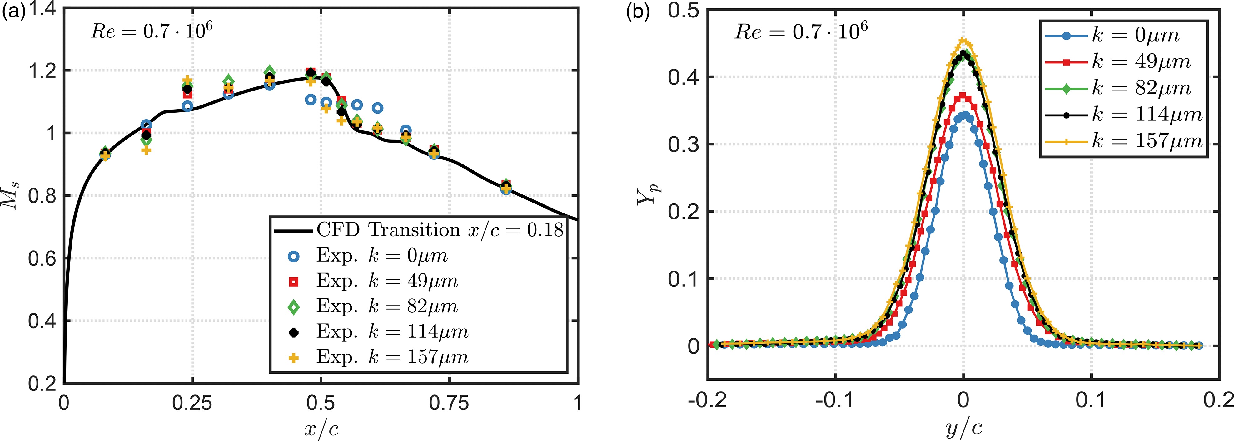
The roughness elements alters the aerofoil loss. To assess the change, linear traverses were performed half a chord downstream of the aerofoil. Figure 5b presents the measured wake loss traverses Yp for all the trip heights. The total pressure loss of the smooth blade is between 25% and 42% lower than for any of the trip heights. This can be explained by three different mechanisms. Firstly, the laminar region of the smooth blade covers 44% of the chord, compared with the 18% for the tripped case. The reduction in turbulent wetted area results in reduced boundary layer losses. Secondly, the pre-shock Mach number of the double shock structure is lower than for the single shock structure. As a result, the loss produced across the shockwave system is lower for the laminar case. This can be confirmed by the marginally lower loss in the free-stream. Thirdly, the laminar/transitional SWBLI does not lead to an open separation which would dramatically increase the mixing loss. Instead, a small separation bubble has been idenfitied. These three mechanisms can explain the reduced total pressure loss observed for the smooth blade. The reduction in loss linked to the smooth case contradicts studies such as Szwaba et al., 2019. In those cases, a smaller fraction of chord associated to laminar boundary layer was present and large separations were observed consequence of the transitional SWBLI, resulting in an overall opposite effect.

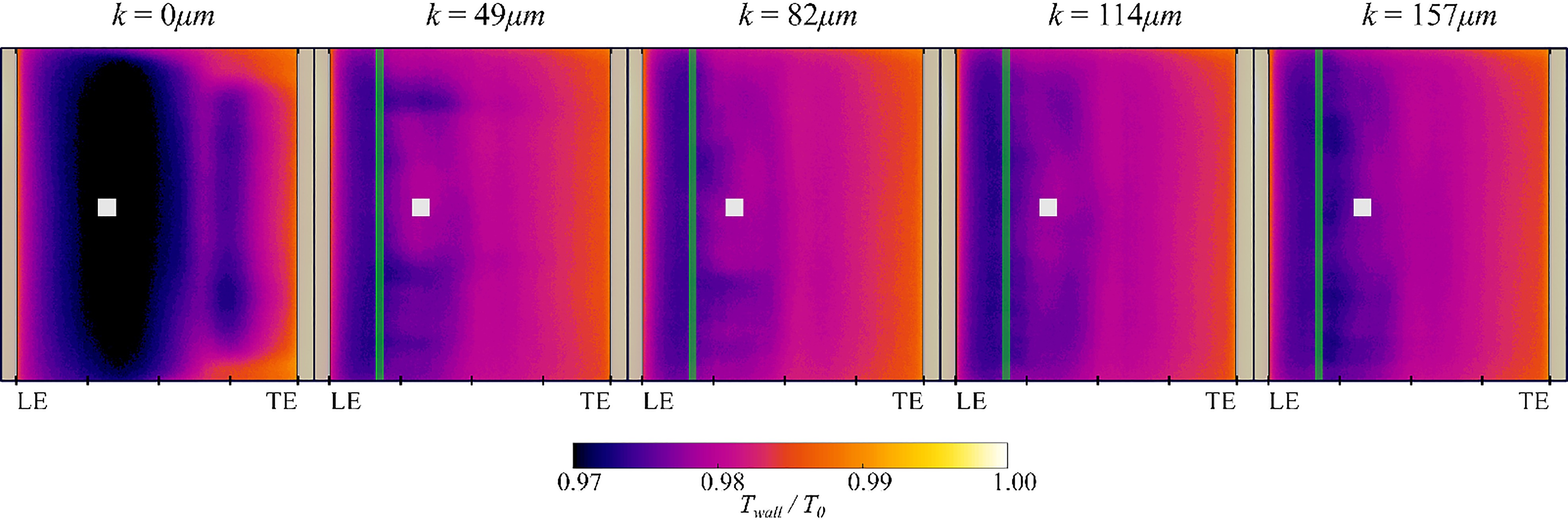
For the roughness heights located within the loss plateau, k=82μm and k=114μm, the loss wakes overlap and a constant increase in loss of 37% is found. As the roughness height drops below the critical value kcrit, transition is successfully induced by the trip but the completion of the transition is delayed. As a result, the turbulent wetted area is reduced leading to an overall smaller increase in loss of 25% relative to the smooth case. For roughness heights larger than the boundary layer (k=157μm in Figure 5b), the fraction of the free-stream adjacent to the boundary layer is disturbed by the trip, resulting in a further 5% increase in loss. The results presented here show that the proposed methodology successfully designs a boundary layer trip with transition at the desired location and with predictable constant loss, as it lays in the middle of the loss plateau.

Reynolds number sensitivity

As the Reynolds number increases, the transition onset is expected to move upstream. The low order model predicts the transition point of the smooth blade to move by only 2% chord. As a result, laminar/transitional SWBLI are expected for the range of Reynolds numbers tested. The distributions of isentropic Mach number shown in Figure 7a for the smooth blade confirms the laminar/transitional nature of the SWBLI. As the Reynolds number increases the second shock moves upstream and the strength of the shock increases. This suggests that the boundary layer at high Reynolds number is able to further withstand the pressure rise imposed by the shockwave, reducing the length of the separation bubble. At high Reynolds number, the wall-temperature presented in Figure 8 does not show a second cold area near; area which was previously associated to a separation bubble. To confirm the laminar nature of the boundary layer, the recovery factor was calculated at ■. For the three lowest Reynolds numbers, the estimated r≈86 approached the theoretical laminar vale. For the highest Reynolds number, an higher recovery was estimated r≈87, which could indicate that a transitional.

Figure 7.

Effect of Reynolds number on (a) isentropic Mach number, (b) loss exit profiles for k=0μm.

Figure 8.

Effect of Reynolds number on blade wall temperature for k=0μm.

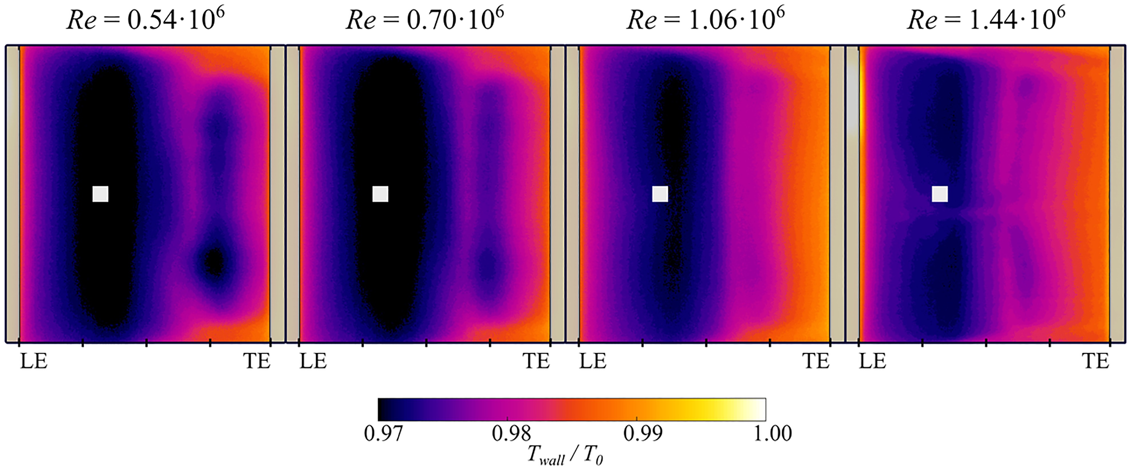
The loss in the free-stream region for the smooth airfoil is independent of the Reynolds number, although it is not visible in Figure 7b because of the scale. This loss is associated to the shockwave losses, which depends on the strength and structure of the shockwave system. As the Mach number and number of shocks remains virtually the same for the range of Reynolds number tested, the shock loss remains unchanged. The length of the separation bubble and the thickness of the boundary layer decrease at high Reynolds number. As a result, the mixing and boundary layer losses decrease with a rise in Reynolds number.

For the nominal trip height of k=82μm, a turbulent SWBLI interaction is observed in Figure 9a for all Reynolds numbers tested. The isentropic Mach number distribution follows closely the design intent shape. For Reynolds numbers Re≥0.7×6 the topology of the non-dimensional temperature presented in Figure 10 remains the same. This topology is characteristic of the turbulent SWBLI and recovery factors indicative of turbulent boundary layer r≈0.89 were measured at ■. For these Reynolds numbers, the nominal roughness height lays within the loss plateau and the surface length based roughness Reynolds number Resk≥105. Although the roughness Reynolds number is high enough to ensure a loss plateau (Resk≥105) at the lowest Reynolds number, the nominal height is smaller than the estimated critical roughness. As a result, complete transition is not expected at the trip for the lowest Reynolds number. To confirm the hypothesis, the recovery factor is calculated at the two locations indicated in Figure 10. Values of r≈0.87 and r≈0.88 indicative of transitional flow were estimated at ♢ and ■, respectively. The heterogeneous recovery factor highlights the relevance of the reliable and homogeneous application of sparse roughness elements to the aerofoil of interest.

Figure 9.

Effect of Reynolds number on (a) isentropic Mach number, (b) loss exit profiles for k=82μm.

Figure 10.

Effect of Reynolds number on blade wall temperature for k=82μm.

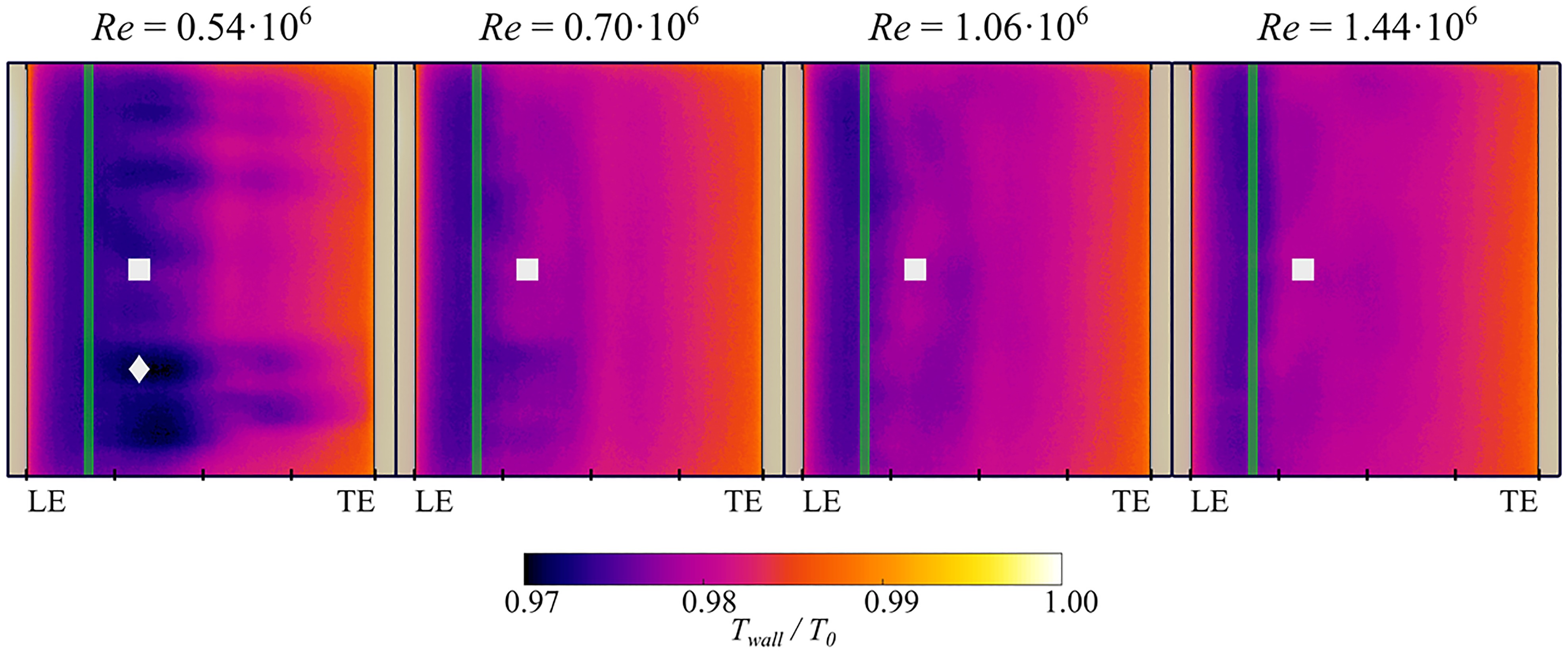
As the Reynolds number increases from Re=0.54×106 to Re=0.7×106, the loss shown in the wake traverse (Figure 9b) increases slightly. The shockwave structure for these Reynolds number is the same. However, Figure 10 highlights the delayed transition at Re=0.54×106 with turbulent flow being reached approximately 15% chord later. This reduction in turbulent wetted area, exchanged for lower loss laminar flow, results in 2.5% reduction in loss at Re=0.54×106. Once the trip is effective, an increase in Reynolds number results in lower boundary layer loss as would be expected from a turbulent boundary layer, reducing the overall loss of the blade.

Revised roughness relation

The Reynolds number and roughness sweeps performed for this transonic aerofoil enables the revision of roughness sizing correlations originally proposed by Braslow et al. (1966). Figure 11a presents the evolution of mass flow averaged total pressure loss as a function of the chord based Reynolds number Re and the roughness height k. Two different behaviours can be observed for constant roughness heights. For a given boundary layer state ahead of the shock (either laminar or turbulent), an increase in Reynolds number results in a gradual decrease in loss. This can be observed for k=0μm and k=157μm where the boundary layer is consistently laminar and turbulent across the Reynolds number range, respectively. For the smallest roughness height k=49μm the boundary layer remains laminar for the two lowest Reynolds number due to the ineffective trip. As a result, an increase in Reynolds number reduces the loss. As the Reynolds number increases enough, the trip becomes effective and an abrupt increase in loss is observed. Once the trip is effective, a further increase in Reynolds number results in a loss reduction. This behaviour is also observed for k=82μm and k=114μm. Due to the higher effective roughness height based Reynolds number Rek, the effectiveness of the trip occurs at a lower chord based Reynolds number.

Figure 11.

Effect of: (a) Reynolds number (b) roughness Reynolds number on total pressure loss.

Figure 11b presents the relation between the total pressure loss, the roughness height based Reynolds number Re_k and the roughness surface distance based Reynolds number Re_sk. For Re_sk ≥10⁵ there exists a plateau of loss with roughness height (or equivalent Re_k). This agrees with the threshold value reported by Braslow et al. 1966. The same authors suggested a minimum value of Re_k,crit ≈ 600 to enter in the plateau. The current dataset suggest that Re_k,crit ≈ 600 is rather conservative, however, it ensures a height independent loss. The critical roughness Reynolds number could be narrowed down by increasing the resolution of roughness heights test, nevertheless this was out of the scope of this work. For all Re_sk tested, a significant increase in loss is observed for very large Re_k. This abrupt rise is linked to roughness heights larger than the boundary layer thickness. The latter agrees with the original methodology of the Braslow et al. 1966. This section has shown the validity of the trip sizing methodology adopted for this blade representative aerofoil. This reinforces the confidence on the application of the proposed methodology to the three-dimensional rotor blade.

Conclusions

This paper proposed the use of an inexpensive and robust flow control method for the suction side of a fan blade. Design guidelines were given for the location and height of the discrete roughness elements used to control the boundary layer state. The method aims at reducing the risk of low Reynolds number experimental fan rig testing.

This paper presented a rapid experimental validation methodology to ensure and de-risk the application of the boundary layer trips to 3D rig blades. The methodology and experimental setup were designed to maximise the control over the experiment, minimise the sources of uncertainty, increase the pace of experimental testing and maximise the range of geometries and operating conditions tested within a modest variable-density wind tunnel.

The experimental methodology was successfully applied to a generic aerofoil representative of a fan tip section. The experimental method was proven to be able to reproduce boundary layers and pressure distributions representative of a 1/10 subscale model. The experiments showed the presence of laminar SWBLI for the baseline untreated blade.

The measurements confirmed that the boundary layer trip successfully fixed transition on the subscale model at the location representative of full-scale blade. The experimental results showed that the trip methodology induced transition with minimum extra blade loss.

The promotion of transition upstream of the shock wave was shown to alter the shock structure. This highlights the importance of conditioning boundary layers in low Reynolds number fan rig testing.

Nomenclature