Case description

The investigated TUDa-GLR-OpenStage is a single-stage high-speed axial compressor, which represents a typical front stage of a high-pressure compressor in a commercial turbofan engine. The compressor stage consists of a blisk rotor with radially stacked CDA-airfoils, a stator with optimized 3D shapes, and an outlet guide vane (OGV) that straightens the flow. The rotor is originally designed by MTU and first tested in 1994. It has been investigated extensively in a series of previous experimental and numerical works (Hoeger et al., 1999; Bergner et al., 2006; Muller et al., 2011). The rotor blades are highly cambered near the hub and thin near the tip. The running tip gap size is approximately 0.75 mm at the design condition, and the hub fillet radius is 5 mm. The stator is designed conjointly between the GLR and the German Aerospace Center (DLR). It is optimized via an automated multi-objective optimization process to suppress the separation size (Bakhtiari et al., 2015). The stator blades have a forward sweep feature near both endwalls and a bow feature towards the pressure surface near the casing. The shapes of the fillets at both endwalls are prescribed by a digitized geometry file. More details about the investigated stage are summarized in Table 1.

Test rig

The TUDa-GLR-OpenStage was tested on the transonic compressor rig of GLR, which can measure the steady-state performance, the aerodynamic instabilities and the blade vibration levels of the compressors. The schematic of the test facility is shown in Figure 1. The inlet flow passes through an inlet throttle, a settling chamber and a mass flow measurement section before reaching the compressor core. The compressor is driven by a DC motor with a gearbox. Shaft input torque and rotor speed is measured using a torque meter.

Figure 1.

Illustration of TUDa-GLR-OpenStage test rig.

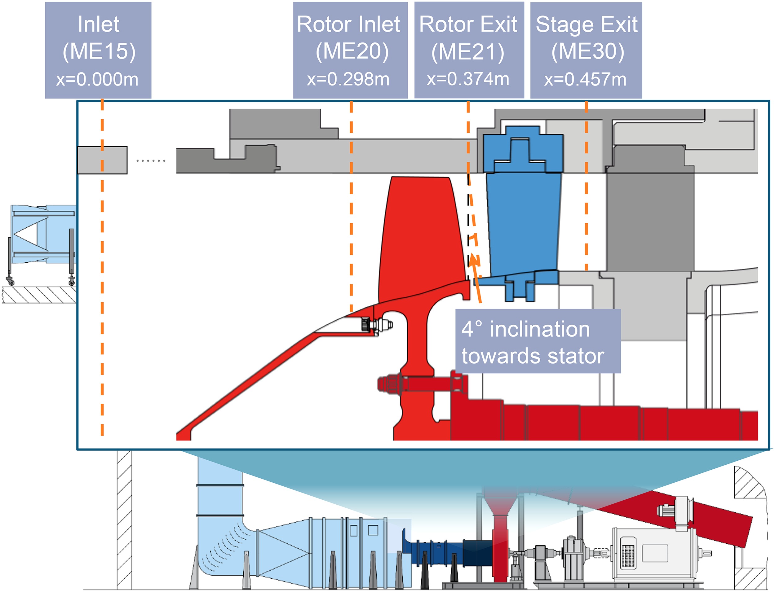
The measurement sections of the compressor are also marked in Figure 1. At the stage inlet section (ME15), radial profiles of total pressure and total temperature are measured. At the rotor exit section (ME21), radial profiles of total pressure and absolute Mach number components are available. At the stage exit section (ME30), 2D distributions of total pressure and total temperature are acquired. The total pressure ratio and total temperature ratio characteristics are calculated by the area-averaged probe data at sections ME15 and ME30; the isentropic efficiency is calculated using the probe-based total pressure ratio and the shaft power. For a fair comparison between the experiment and CFD, the isentropic efficiency from CFD is calculated based on the area-averaged pressure ratio and the mass-averaged temperature ratio. Calculations of the measurement uncertainty along with the measured data are detailed in the concurrent experimental work (Klausmann et al., 2021).

The measurements were performed at 100%, 80% and 65% design speed. This work mainly focuses on the 100% design speed at the peak-efficiency (PE) condition $\lpar m = 16.00 \pm 0.02\; {\rm kg/s}\rpar $ and the near-stall (NS) condition $\lpar m = 14.78 \pm 0.02\; {\rm kg/s}\rpar $.

CFD solvers

In this work, two widely used commercial RANS flow solvers are adopted: Ansys CFX 20.1 and Numeca FineTurbo 14.1.

Ansys CFX uses an element-based finite volume method to discretize the RANS equations based on unstructured meshes. The diffusion term is discretized by the second-order accurate central scheme, and the advection term is discretized by the second-order accurate high resolution scheme. The temporal discretization is achieved by the second-order accurate backward Euler scheme. The linearized equations are solved by the Incomplete Lower Upper (ILU) factorization technique, which is accelerated by an algebraic multigrid method. A pseudo time-stepping algorithm with an automatic time scale technique is used for steady-state calculations. For best-practice of turbomachinery simulation, the updated Menter $k-\omega $ shear stress transport (SST) turbulence model (Menter et al., 2003) (i.e., “SST-2003” (Rumsey, 2021)) is recommended. The Spalart-Allmaras (SA) turbulence model (Spalart and Allmaras, 1994) (i.e., “SA-noft2” (Rumsey, 2021)) is also available. More details about the solver can be found in its user guide (ANSYS, 2021).

Numeca FineTurbo discretizes the RANS equations using a cell-centered control volume approach based on structured meshes. The diffusion term is discretized by the second-order accurate central scheme. The advection term is discretized by either the central scheme with a Jameson-Schmidt-Turkel (JST) type dissipation term (Jameson et al., 1981) or the upwind scheme using flux difference splitting from Roe (1981), both of which are second-order accurate. The temporal discretization is achieved by the explicit fourth-order accurate Runge-Kutta integration scheme. For steady-state cases, the pseudo time-stepping algorithm is used. Local time stepping, implicit residual smoothing, and multigrid techniques are applied to accelerate convergence. The modified SA turbulence model (Ashford, 1996) (i.e., “SA-fv3-noft2”1 [1] (Rumsey, 2021)) is set as the default for turbomachinery simulations. Other turbulence models including the modified SARC model (Shur et al., 2000) (i.e., “SA-RC-fv3-noft2” (Rumsey, 2021)), the original SST model (Menter, 1994) (i.e., “SST” (Rumsey, 2021)) and the simplified baseline EARSM model (Menter et al., 2012) are also available. More details of the solver can be found in its user guide (NUMECA International, 2021).

Flow domain, boundary conditions and grids

The simulation is conducted by using a single-passage flow domain with the circumferentially periodic boundary condition, as illustrated in Figure 2a. The inlet plane is set at the stage inlet section ME15. The measured total pressure and total temperature profiles are used to prescribe the inlet boundary condition. In addition, the inlet flow direction is axial; the turbulence intensity and turbulence length scale are estimated as 4% and 0.09 mm respectively, which are equivalent to an eddy viscosity ratio of 35. At the rotor-stator and the stator-OGV interface, a mixing plane boundary condition (specifically, “Stage (Mixing-Plane)” with “Constant Total Pressure” as downstream velocity constraint for Ansys CFX; “Full Non-Matching Mixing Plane” for Numeca FineTurbo) is used. The outlet boundary is set at the location about 1.5 times the compressor core axial length downstream of the OGV. A radial equivalent backpressure is assigned at the outlet boundary, but a constant backpressure value can also be used since the outlet flow is turned to the axial direction by the OGV. When approaching the stall limit, a step increase of backpressure of 200 Pa is used. The last converged point is taken as the numerical “stall” point.

Figure 2.

Illustration of TUDa-GLR-OpenStage CFD model. (a) Flow domain and boundary conditions (b) Grid topology (c) Visualization of the Medium grid at mid-span.

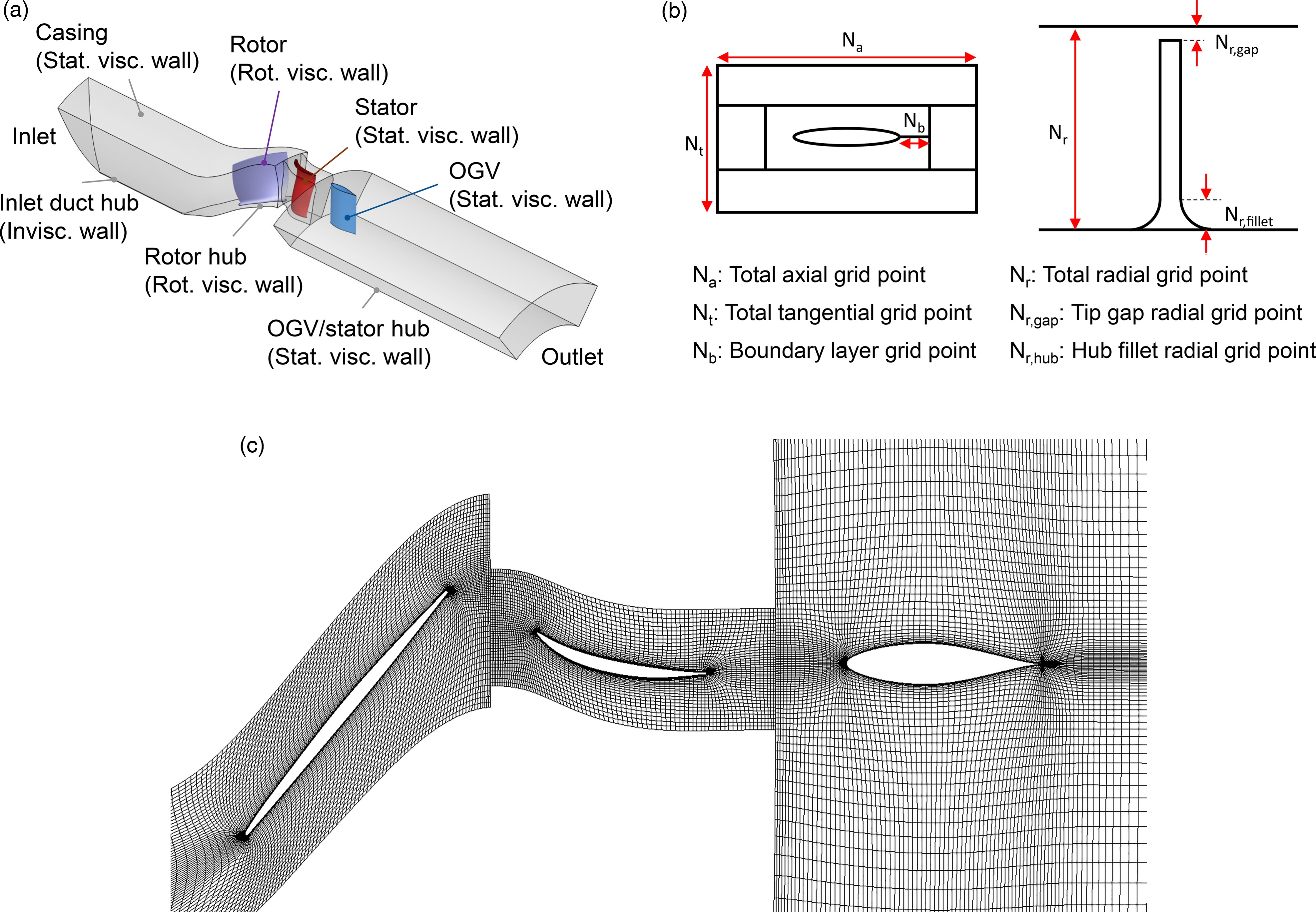
The flow domain is discretized by hexahedron grids with an O4H topology, which are generated by using the Numeca AutoGrid5. In total, five sets of rotor and stator grids with different grid densities are generated. The mesh refinement is achieved by uniformly increasing the grid number to about 1.5 times in all dimensions, while the first layer grid displacement is kept the same at an area-averaged $y^ + $ value around 1.1. Endwall features including gaps and fillets of the rotor and the stator are considered in the grid. Details of the grids are summarized in Table 2, and the grid topology is illustrated in Figure 2b. The OGV is meshed by a hexahedron grid with 0.8 million grid nodes, which has a similar grid density to the Medium grid of the rotor and the stator. Since the OGV does not have a pronounced effect on the upstream flow field, its grid density is kept the same throughout the paper. For a better representation of the computational grid, the Medium grid at the mid-span is presented in Figure 2c.

Effect of grid density

In this section, five sets of uniformly refined grids (detailed in Table 2) are adopted to investigate the effect of grid density. Unless stated elsewhere, the rest of the numerical settings are kept the same, including the Ansys CFX solver, the SST turbulence model and the mixing plane rotor-stator interface model.

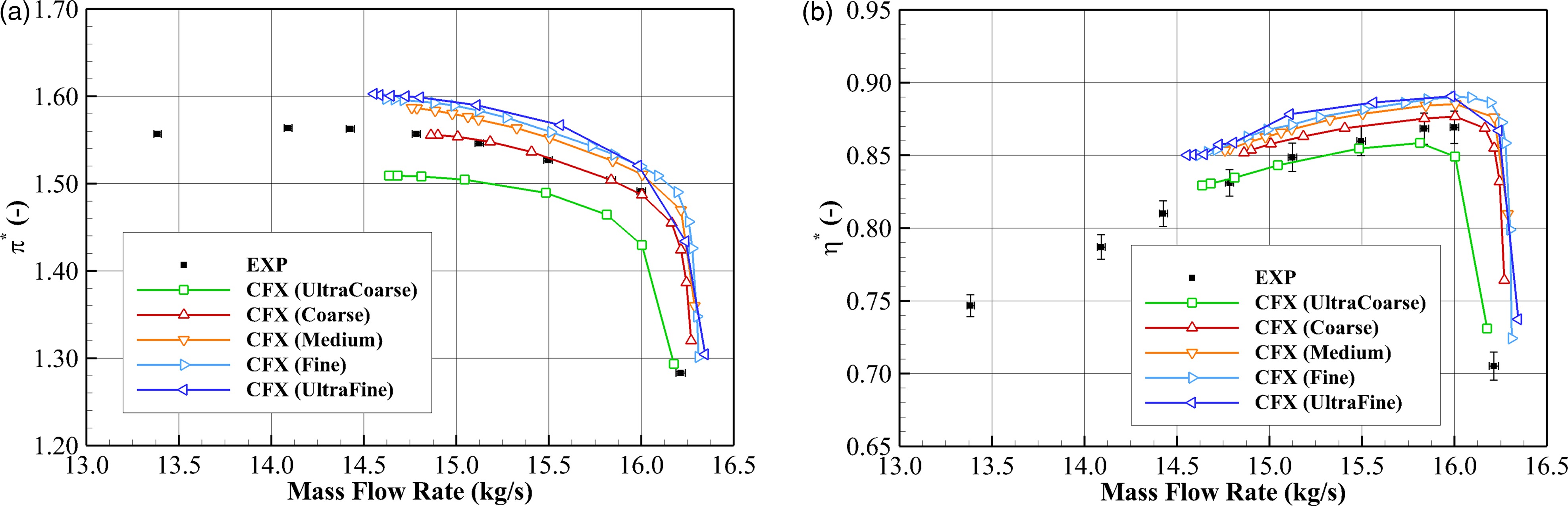
The stage performance characteristics at the design speed are presented in Figure 3, where the simulation results are represented by curves with open symbols, and the experimental data are denoted by solid squares with error bars. As the grid density increases, the characteristic curves gradually translate towards the top-right corner (i.e., higher pressure ratio, efficiency and mass flow rate; similar slopes of pressure ratio and efficiency curve). Excluding the UltraCoarse grid result, the stable flow range $\lpar {\rm SFR} = \lpar m_c-m_s\rpar {\rm /}m_c \times 100\percnt \rpar $ increases with the grid density, from 8.7% of the Coarse grid result to 11.2% of the UltraFine grid result. When refining the grid to the Fine and UltraFine levels, the variation of pressure ratio and efficiency are within 0.01 and 0.1% respectively, indicating a grid-independent result. Note that although the results from the Coarse grid results match the best with the measured data, they are subjected to pronounced discretization error and thus cannot be taken as evidence of a good validation.

Figure 3.

Effect of grid density on predicting the TUDa-GLR-OpenStage performance characteristics: (a) total pressure ratio and (b) isentropic efficiency.

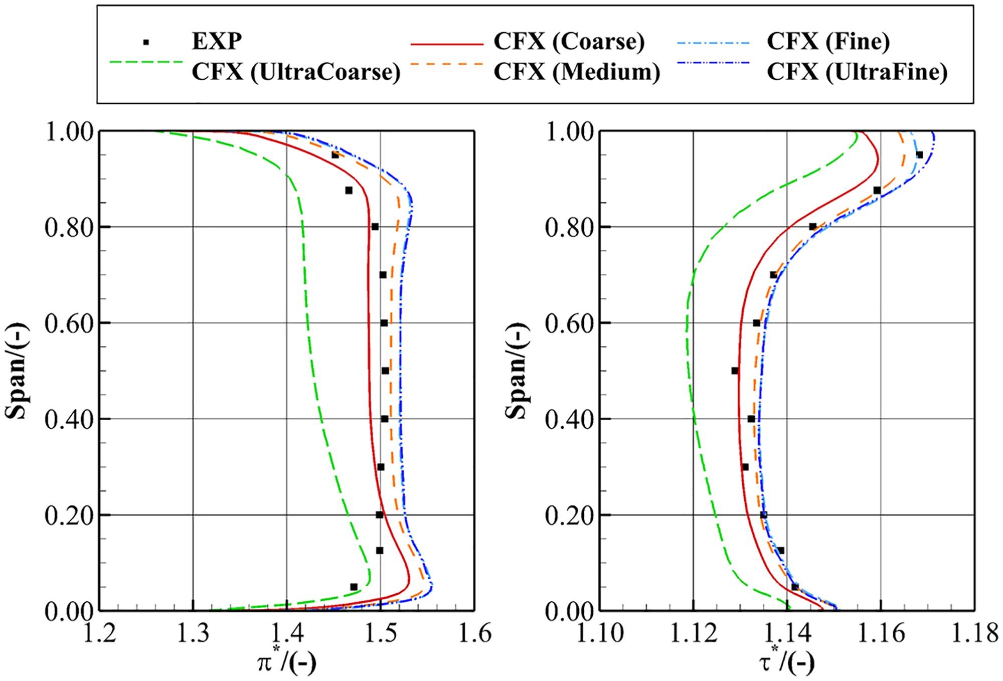
To examine the effect of grid density on the flow fields, the circumferentially mass-averaged radial profiles downstream of the stator are presented in Figure 4. In these plots, curves represent the numerical results obtained from the five grids, and solid squares denote the experimental results. For simplicity, only the PE results are presented. Results show that grid refinement leads to an increased total pressure ratio and total temperature ratio, especially at the upper 20% span. The Fine and UltraFine results are almost overlapping with each other, indicating grid independence has been achieved. However, they over-predict the total pressure ratio in the upper and lower 20% spans near the endwalls. Such a deficiency can be caused by the deficiency of the turbulence model, the deficiency of the mixing plane model, or plausible geometric uncertainties and errors. These factors will be examined later.

Figure 4.

Effect of grid density on predicting the circumferentially mass-averaged radial profiles at the stage exit (ME30) at the PE condition.

Following the concept of Roache (1998), the grid discretization error scales with ${\rm \Delta }^n$ when using a $n_{th}$ -order accurate advection scheme, where ${\rm \Delta } = \lpar 1{\rm /}N_g\rpar ^{1{\rm /}3}$ is the nominal grid spacing with $N_g$ the total number of grid points. For the second-order accurate schemes used in this work, a parabola can be fitted through the simulation results from different grids, i.e., $q = k{\rm \Delta }^2 + q_{{\rm ideal}}$, where k measures the grid convergence rate and $q_{{\rm ideal}}$ is the ideal simulation result free of discretization error. To check the grid convergence of different turbulence models and different solvers, the total pressure ratio and efficiency at the PE condition are plotted against ${\rm \Delta }$ in Figure 5. In these plots, the solid square with error bars at ${\rm \Delta } = 0$ denotes the experimental data, the rest scatters represent the simulation data obtained from the five grids, and the curves are the least-squares fitted parabolas.

Figure 5.

Grid convergence of TUDa-GLR-OpenStage at the PE condition using different turbulence models implemented in different solvers: (a) total pressure ratio and (b) isentropic efficiency.

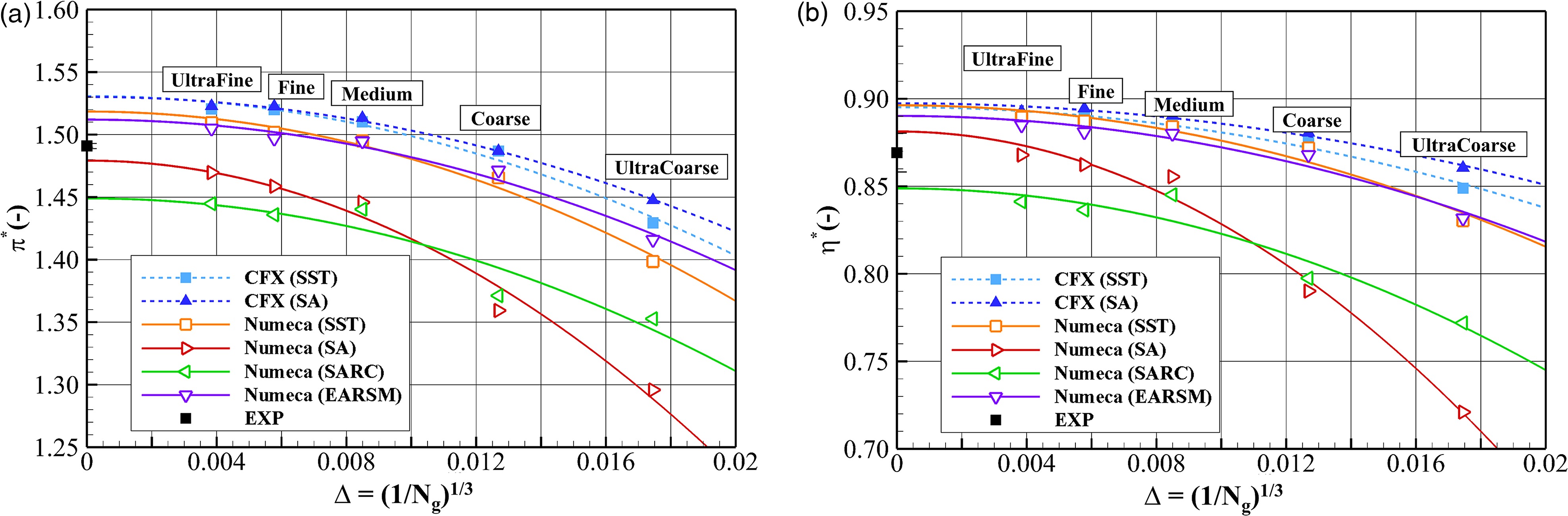
Comparing the investigated five grids, the choice of grid density yields a 7% relative (to experiment) variation in total pressure ratio and a 7% absolute variation in isentropic efficiency. The discretization errors of the Fine grid, i.e., $\vert {q_{{\rm ideal}}-q_{{\rm Fine}}} \vert $, are about 0.01 in total pressure ratio and 0.5% in efficiency, which is adequately small. Therefore, the Fine grid will be used in later sections of the paper.

Comparing the investigated four turbulence models implemented in the two solvers, the choice of turbulence model yields a 5% relative variation in total pressure ratio and a 5% absolute variation in isentropic efficiency for the discretization-error-free values $q_{{\rm ideal}}$ at ${\rm \Delta } = 0$. Specifically, the CFX(SST) method and the CFX(SA) method show similar prediction results, indicating both the SST-2003 and the SA-noft2 model are equally accurate in predicting this case. The Numeca(SA) method is evidently more sensitive to the grid density than the rest turbulence models, which is deduced to be caused by the fv3 version of the SA model.

Effect of Advection Scheme

In this section, the JST central scheme (Jameson et al., 1981) and the Roe upwind scheme (Roe, 1981) are compared with each other, both of which are second-order accurate. The rest of the numerical settings are kept the same, including the Numeca solver, the Fine grid, the SST turbulence model and the mixing plane rotor-stator interface model.

The discretization error related to a second-order accurate advection scheme scales with the square of the grid spacing. Thus, the difference between the schemes is expected to be evident only when a coarse grid is used. In Figure 6a, the grid convergence of different advection schemes on predicting the compressor total pressure ratio at the PE condition is presented. It is confirmed that the choice of advection scheme has a negligible effect when refining the grid to the Fine grid level.

Figure 6.

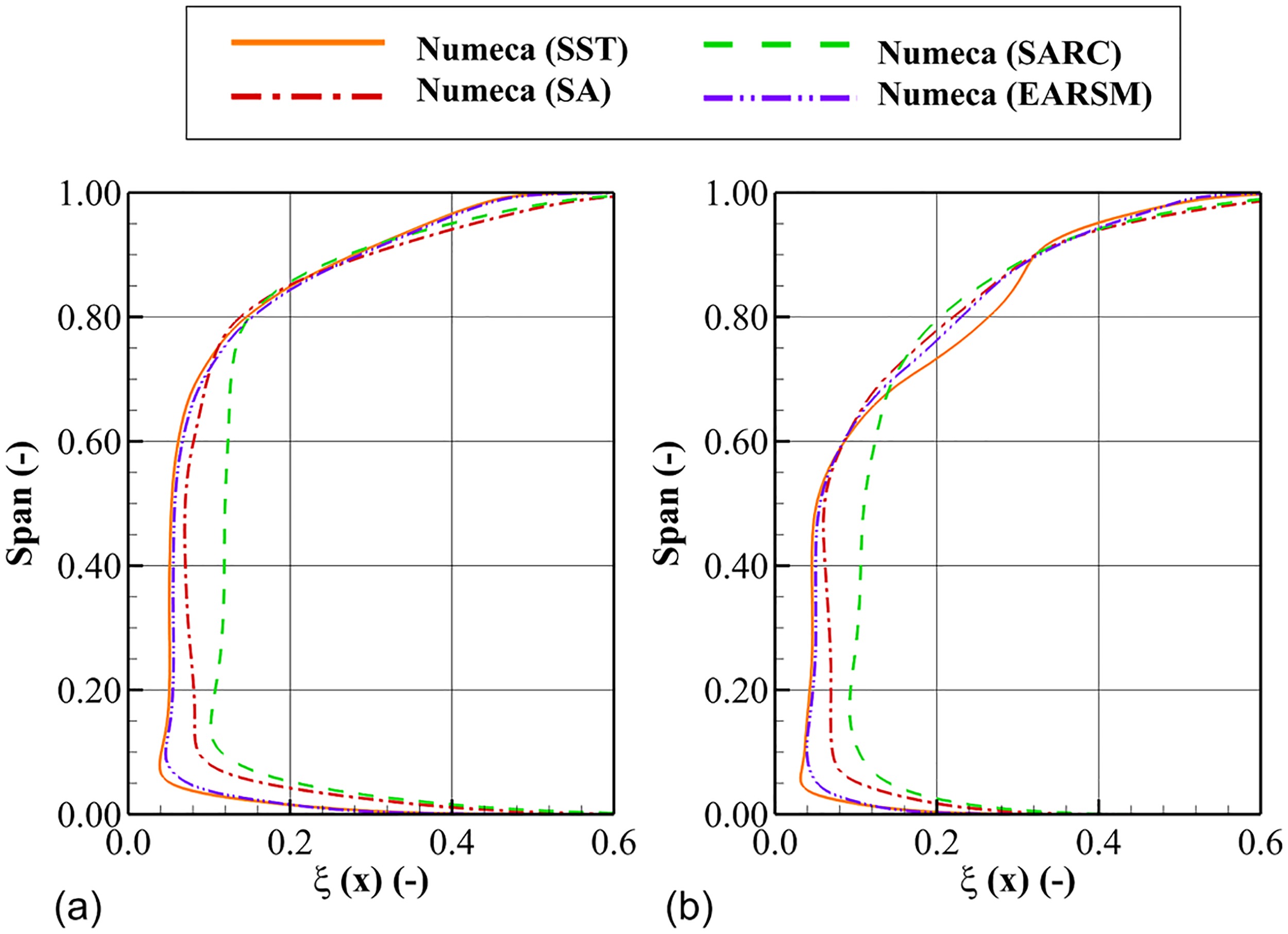
Grid convergence of TUDa-GLR-OpenStage at the PE condition using different advection schemes: (a) total pressure ratio and (b) normalized shock front location at 90% span of the rotor.

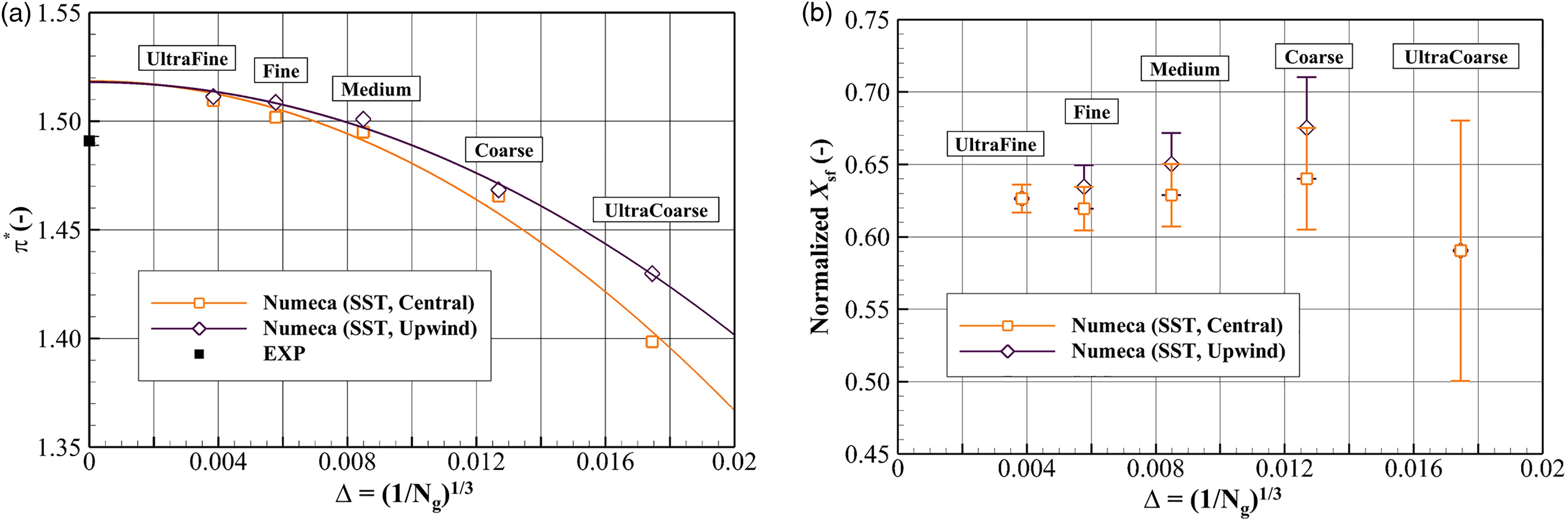
For a more detailed comparison, the grid convergence of different advection schemes on predicting the rotor suction surface shock front location is presented in Figure 6b. Here, the shock front is defined at the grid point where $\partial ^2p{\rm /}\partial x^2$ reaches the maximum, and the fourth-order central finite difference method is used to calculate this derivative. The axial distance between the leading edge and the derived shock front location is then normalized by the axial chord length at the corresponding span, yielding the normalized shock front location $X_{sf}$. To represent the local grid density, the grid spacing of the adjacent grid cells is denoted by the error bars. Results show that the central scheme predicts the shock front slightly more upstream (i.e., by one grid spacing) than that of the upwind scheme when using the Coarse, Medium or Fine grid. This difference becomes indistinguishable when refining the grid to the UltraFine grid level.

For best practice, it is the choice of grid density rather than the choice of advection scheme that should be paid more attention to. Although any advection scheme can achieve an accurate prediction once the grid independence requirement has been met, a high-order scheme is still favorable in terms of computational cost.

Effect of turbulence model

In this section, four turbulence models namely SST, SA, SARC and EARSM are compared with each other. The rest of the numerical settings are kept the same, including the Numeca solver with the central advection scheme, the Fine grid and the mixing plane rotor-stator interface model.

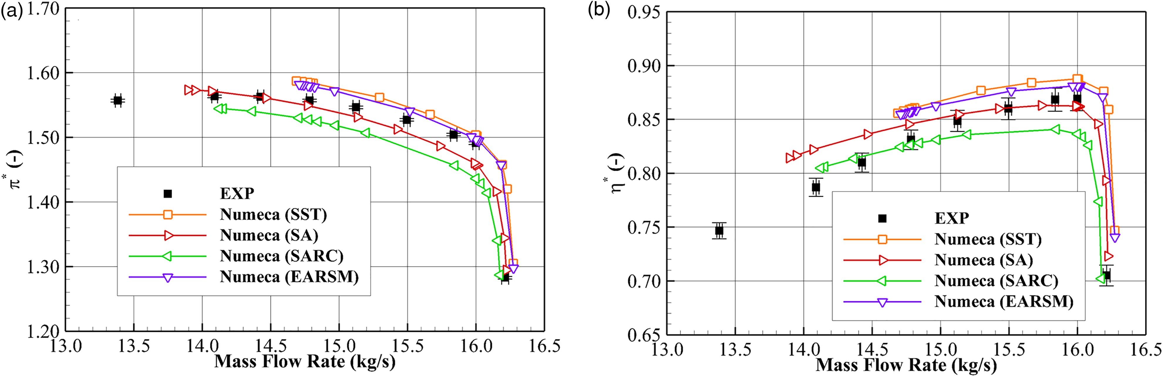
The stage performance characteristics at the design speed are compared with experimental data in Figure 7, where the measured data are represented by solid squares with error bars, and the simulation data are denoted by lines with scatters. In general, the SA model and the EARSM model predict the best agreement with the measured data. The SA model reproduces the stall margin2 [2] (SFR = 13.0% for the experiment; SFR = 14.3% for the SA prediction), the NS pressure ratio and the PE efficiency; however, the PE pressure ratio is under-predicted and the NS efficiency is over-predicted. The EARSM model accurately predicts the PE pressure ratio, but it under-predicts the stall margin (SFR = 9.6%) and slightly over-predicts the NS pressure ratio and the overall efficiency. The SST model predicts the highest pressure ratio and efficiency, but it is close to the EARSM results. The SARC model predicts the lowest pressure ratio and efficiency, which shows the least agreement with the measured data.

Figure 7.

Effect of turbulence model on predicting the TUDa-GLR-OpenStage performance characteristics: (a) total pressure ratio and (b) isentropic efficiency.

For further comparisons between the four turbulence models, the radial profiles at the rotor exit and the stage exit are examined in Figure 8. In these plots, simulation results are represented by lines, and the measured data are denoted by solid squares.

Figure 8.

Effect of turbulence model on predicting the circumferentially mass-averaged radial profiles. (a) PE, rotor exit (ME21) (b) PE, stage exit (ME30) (c) NS, rotor exit (ME21) (d) NS, stage exit (ME30).

At the PE condition, both the SA model and the SARC model under-predict the pressure ratio and the flow angle at the rotor exit below 80% span, as shown in Figure 8a. Such deficiencies generally propagate to the stage exit shown in Figure 8b, which accounts for the under-prediction of the overall stage pressure ratio at the PE condition. The EARSM model and the SST model slightly over-predict the rotor exit pressure ratio above the 80% span and the rotor exit flow angle at full span, as presented in Figure 8a. At the stage exit shown in Figure 8b, the near-tip over-prediction of pressure ratio in the rotor passage is propagated to the stage exit; in addition, the near-hub over-prediction of pressure ratio arises, which is induced in the stator passage. These deficiencies of the endwall pressure ratio prediction, however, are too small to be observed in the overall stage pressure ratio shown in Figure 7a.

At the NS condition, the SA model predicts the most accurate pressure ratio profile at the stage exit, as shown in Figure 8d; the SARC model still under-predicts the pressure ratio at most spans, whereas the SST model and the EARSM model over-predict it especially near the endwalls. The shapes of all the pressure ratio profiles at the stage exit are similar to that at the rotor exit shown in Figure 8c, except that the SST result shows a total pressure loss near 80% span at the stage exit plane. This drop of total pressure corresponds to an excessive prediction of the corner separation size in the stator, as will be shown later. In terms of the stage exit total temperature ratio shown in Figure 8d, the EARSM model and the SST model show the best agreement with the measured data, whereas the SA model and the SARC model slightly under-predict it.

To complement the validation on the radial profiles, the total pressure ratio contours at the stage exit are presented in Figure 9. In these plots, the top row and the bottom row represent the PE condition and the NS condition, respectively; the columns from left to right represent the experiment, SST, SA, SARC and EARSM results.

Figure 9.

Effect of turbulence model on predicting the total pressure ratio contours at the stage exit (ME30).

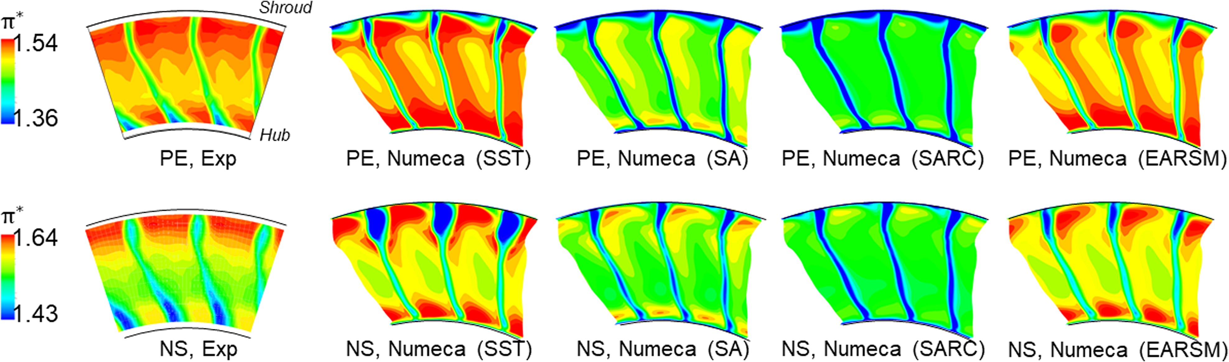
For the experimental results, a hub-suction surface corner separation is observed at both the PE and NS conditions, which is featured by low values of total pressure. As the compressor operates from PE to NS, the separation size increases. This corner separation, however, is not reproduced by any of the simulation results, leading to the near-hub over-prediction of the total pressure ratio observed previously in Figure 8b and d.

Among the simulation results, the SARC model and the SST model predict the lowest and highest overall total pressure ratio, respectively, which deviates from the measured data the most. The SST model also over-predicts the near-tip trailing edge separation size at the NS condition. Despite the EARSM model and the SA model predicting the best agreement with the measured data, evident differences still persist. Further investigations regarding the effect of the rotor-stator interface model and the effect of geometric uncertainties and errors (e.g., stator hub cavity leakage flow) are needed to improve the prediction accuracy.

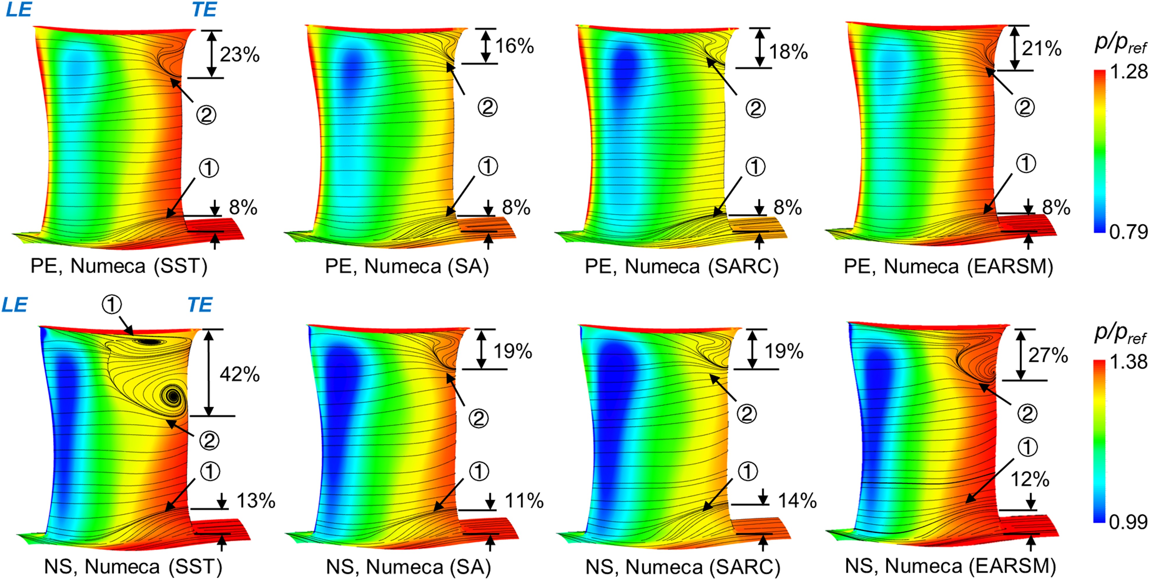
To compare the four turbulence models in predicting the rotor flow field, the static pressure contours superimposed with the surface limiting streamlines on the rotor suction surface are presented in Figure 10. In general, the rotor flow field is featured by a near-hub corner separation and a near-tip shock-induced separation. When the compressor is throttled towards stall, the shock front moves further upstream, and the sizes of both separation cells increase. Comparing the effect of turbulence models, the SST model predicts the largest separation size, followed by the EARSM, SA and SARC model. In particular, the near-tip shock-induced separation is not captured by the SA model at the PE condition, as well as the SARC model at both the PE and NS conditions. Such results imply that the SA and SARC models predict higher eddy viscosity in the rotor passage than the other models, which will be examined latter.

Figure 10.

Static pressure contours and surface limiting streamlines on the hub surface and the suction surface of the rotor; ①: corner separation; ②: shock-induced separation; ③: shock front.

To compare the four turbulence models in predicting the stator flow field, the static pressure contours superimposed with the surface limiting streamlines on the stator suction surface are presented in Figure 11. In general, the stator flow field is featured by a near-hub corner separation and a near-tip trailing edge separation. As the compressor operates toward stall, the sizes of both separation cells increase. Similar to the observations in the rotor flow fields, the SST model predicts the largest separation size, followed by the EARSM, SA and SARC model. In particular, at the NS condition, the SST model predicts a near-tip corner separation that connects with the trailing edge separation. This excessive prediction of separation size is consistent with previous observations in Figures 8d and 9.

Figure 11.

Static pressure contour and surface streamlines on the hub surface and the suction surface of the stator; ①: corner separation; ②: trailing edge separation.

To help understand the loss mechanism predicted by different turbulence models, the loss of efficiency $\xi $ is monitored. The concept of loss of efficiency was originally introduced by Denton (1993) as an overall measure of compressor loss, i.e., $\xi = T_{t\comma e}\lpar S_e-S_i\rpar {\rm /}c_p\lpar T_{t\comma e}-T_{t\comma i}\rpar \approx 1-\eta ^{\ast} $, where $T_{t\comma i}$, $T_{t\comma e}$, $S_i$, $S_e$ are the total temperature and the entropy at the inlet and the exit, respectively. Later, it was extended to a scalar field $\xi \lpar { x}\rpar $ (He and Zheng, 2016), i.e., $\xi \lpar {x}\rpar = T_{t\comma e}\lpar S\lpar {x}\rpar -S_i\rpar {\rm /}c_p\lpar T_{t\comma e}-T_{t\comma i}\rpar $, where $S\lpar { x}\rpar $ is the entropy at an arbitrary location ${x}$.

The radial profiles of $\xi $ at the stage exit (ME30) are presented in Figure 12. For the SST model and the EARSM model, their loss of efficiency profiles almost overlap with each other at the PE condition. However, the SST model predicts a higher loss near the 80% span at the NS condition, which corresponds to the excessive near-tip flow separation observed previously in Figure 11. For the SA model and the SARC model, they predict higher loss than the rest models below 70% span at both operating conditions, indicating the SA model and the SARC model predict a higher level of eddy viscosity and thus stronger skin friction on the blade surfaces. Such an effect on the eddy viscosity field will be confirmed later.

Figure 12.

Circumferentially mass-averaged radial profiles of loss of efficiency at the stage exit (ME30): (a) PE condition; (b) NS condition.

The investigated four turbulence models are all based on the concept of eddy viscosity. To help understand the behavior of the turbulence models further, the turbulent-to-laminar viscosity ratio contours are presented in Figure 13, where each row corresponds to an operating condition, and each column corresponds to a turbulence model. For the compactness of the figure, the inlet duct and the OGV are not shown.

Figure 13.

Circumferentially mass-averaged turbulent-to-laminar viscosity ratio contours.

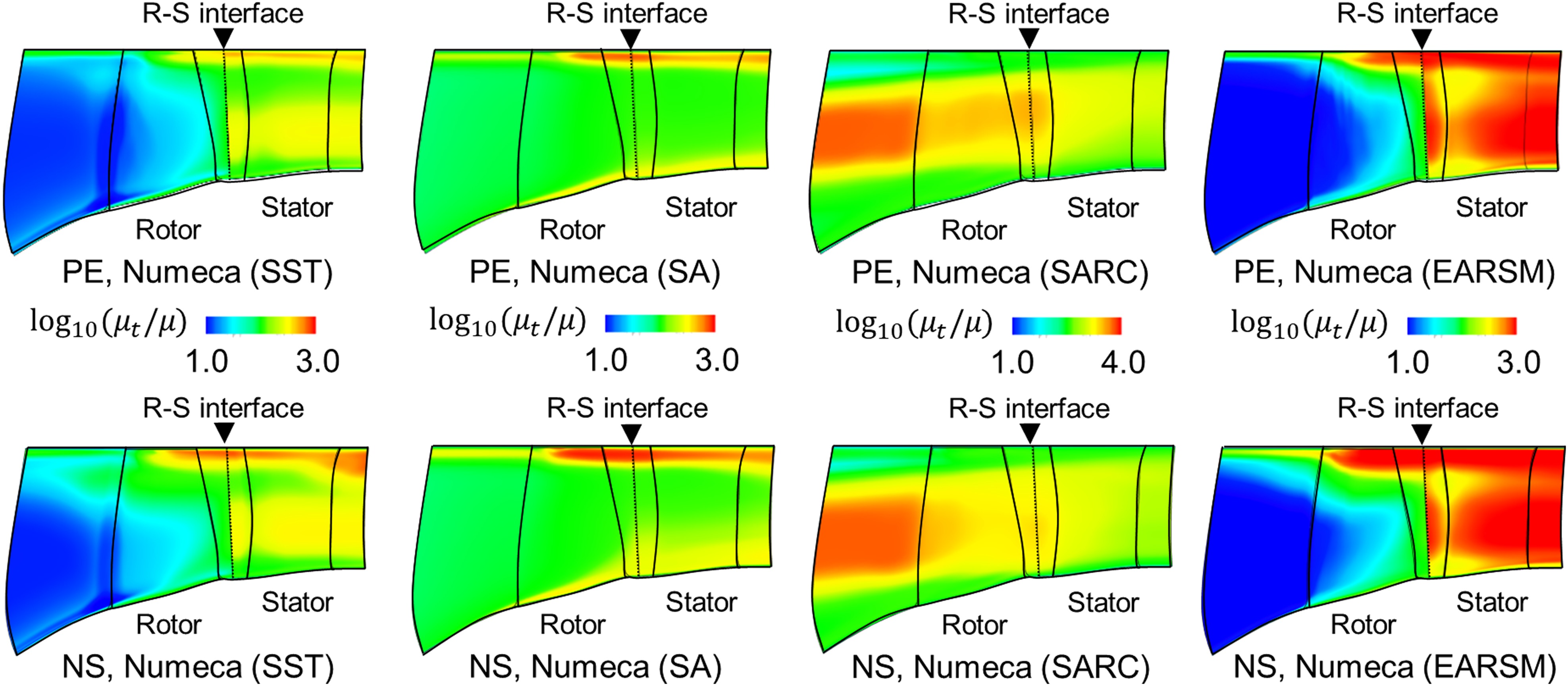
For the two-equation turbulence models SST and EARSM, they are insensitive to the freestream eddy viscosity boundary condition (i.e., $\mu _t{\rm /}\mu = 35$) assigned at the inlet of the simulation domain (not shown), as $\mu _t{\rm /}\mu $ dissipates to a small value before entering the rotor passage. Afterward, $\mu _t{\rm /}\mu $ develops with the rotor blade surface boundary layers in the mid-spans and with the tip leakage separation cell in the near-tip spans; the closer toward the NS condition, the higher the eddy viscosity level in the blade passage. When passing through the mixing plane interface, discontinuity of $\mu _t$ arises. Such a discontinuity is induced by the implementation of the mixing plane: conventionally, the two turbulence model quantities (e.g., k and $\omega $ in this case) are mixed out and thus are conservative across the mixing plane; when converting these quantities back to eddy viscosity (i.e., $\mu _t\sim k{\rm /}\omega $), conservation of $\mu _t$ is not guaranteed. In this case, $\mu _t$ is abruptly increased immediately downstream of the mixing plane, which tends to reduce the separation size in the stator passage. For future research, it is recommended to test a mixing plane model that conserves $\mu _t$ and k across the interface.

For one-equation turbulence models SA and SARC, they are more sensitive to the freestream eddy viscosity as $\mu _t{\rm /}\mu $ increases by an order of magnitude before entering the rotor passage. The reason is that the dissipation term of $\mu _t$ depends purely on the wall distance and high $\mu _t{\rm /}\mu $ values in far-wall regions (e.g., farfield, freestream, etc.) cannot be dissipated effectively. As a result, the one-equation models predict a smaller separation size than the two-equation models in the rotor passage. The SARC model, in particular, predicts excessive values of $\mu _t$ upstream of the rotor passage. In the first place, these results were qualitatively reproduced by using an in-house flow solver (He et al., 2020) to rule out potential coding errors. By checking the formulation of the SARC model, it is found that the $r^{\ast} $ term goes infinitely large, which triples the production term of $\mu _t$ and thus the excessive $\mu _t$ at the inlet. This feature of the SARC model leads to an over-prediction of skin friction loss, an under-prediction of separation size, and hence the least accuracy in predicting the compressor performance and flow fields. Therefore, it is not recommended for axial compressor applications.

Effect of rotor-stator interface model

In this section, the mixing plane rotor-stator interface model typically used in steady simulations is compared with the sliding plane model used in unsteady simulations. The investigation is performed by using the Ansys CFX solver, the Fine grid topology and the SST turbulence model. To reduce the required computational resources, the number of stator blades has been changed from 29 to 32 so that a periodic sector of one rotor blade and two stator blades (1R2S) can be used for the sliding plane model. The time step used in the unsteady simulation corresponds to ${\rm \Delta }t\cdot {\rm BPF} = 48$, and the second-order backward Euler scheme is used for time stepping. The simulation has been performed over 6 rotor revolutions to reach a statistically steady state, and the data obtained in the last blade passing period is used for time averaging.

The stage exit (ME30) radial profiles obtained from the mixing plane method and the time-averaged sliding plane method are compared in Figure 14a. In the first place, the steady-state performances before and after changing the number of stator blades are compared with each other. It shows that both cases have almost the same profiles, indicating the scaling of the stator geometry barely changes the flow physics. Then, the sliding plane result is compared with the mixing plane result. No evident difference is found except that the sliding plane result shows slightly better agreement with the measured total temperature ratio. Such results indicate the mixing plane model is reasonably accurate at the investigated PE and NS conditions. Finally, comparing all CFD results with the measured data, the over-prediction of the stage pressure ratio in the upper and lower 20% span still persists. Such deficiencies are potentially caused by the geometric errors (as will be discussed in the later section) and the non-ability of RANS to sufficiently capture the turbulence effect of endwall flows.

Figure 14.

Effect of rotor-stator interface model on predicting the flow field at the PE condition. (a) Stage exit (ME30) radial profiles (b) Circumferentially mass-averaged viscosity ratio.

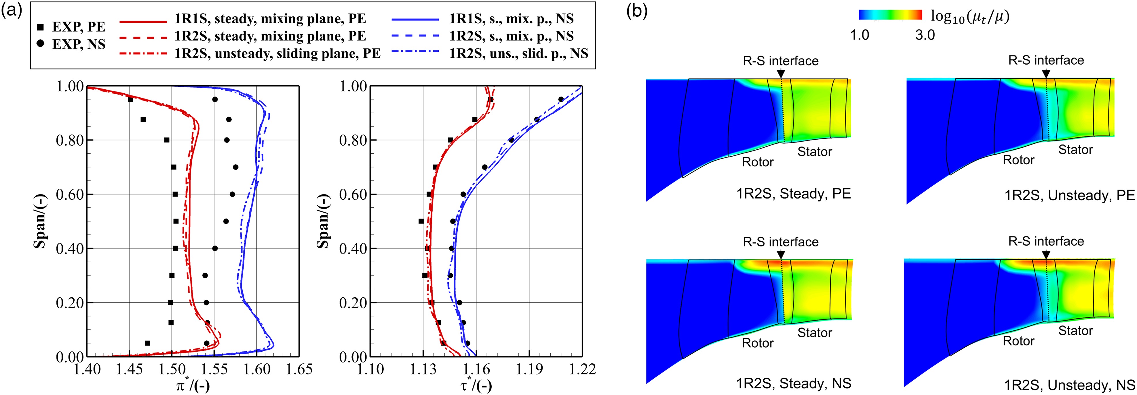
To unveil the effect of the rotor-stator interface model on predicting the eddy viscosity field, the turbulent-to-laminar viscosity ratio contours are presented in Figure 14b. Results show that the mixing plane results have an abrupt increase of $\mu _t$ across the interface, whereas the time-averaged sliding plane results show a continuous distribution of $\mu _t$ across the interface, which is more reasonable. The difference of the overall $\mu _t$ distribution in the stator passage, however, is evident only near the stator leading edge. Such a difference will not have a visible effect on the downstream separation and thus the small difference in the mean flow field.

Effect of rotor running tip gap shape

In the experiment, the rotor running tip gap shape was measured by a capacitive blade tip timing system, and the tip gap size was found to increase by 0.2% $C_t$ when throttling from the PE to the NS condition (Klausmann et al., 2021). To evaluate its effect on the predictions, the measured running tip gap shapes are simulated by using the Numeca solver with the central advection scheme, the Fine grid, the SST turbulence model and the mixing plane rotor-stator interface model. Results show that the difference in the stage total pressure ratio and the stage isentropic efficiency is only within 0.01 and 0.1% at both the PE and the NS conditions, which is consistent with previous research (Berdanier and Key, 2015). Therefore, the error induced by the running tip gap shape can be ignored in this case.

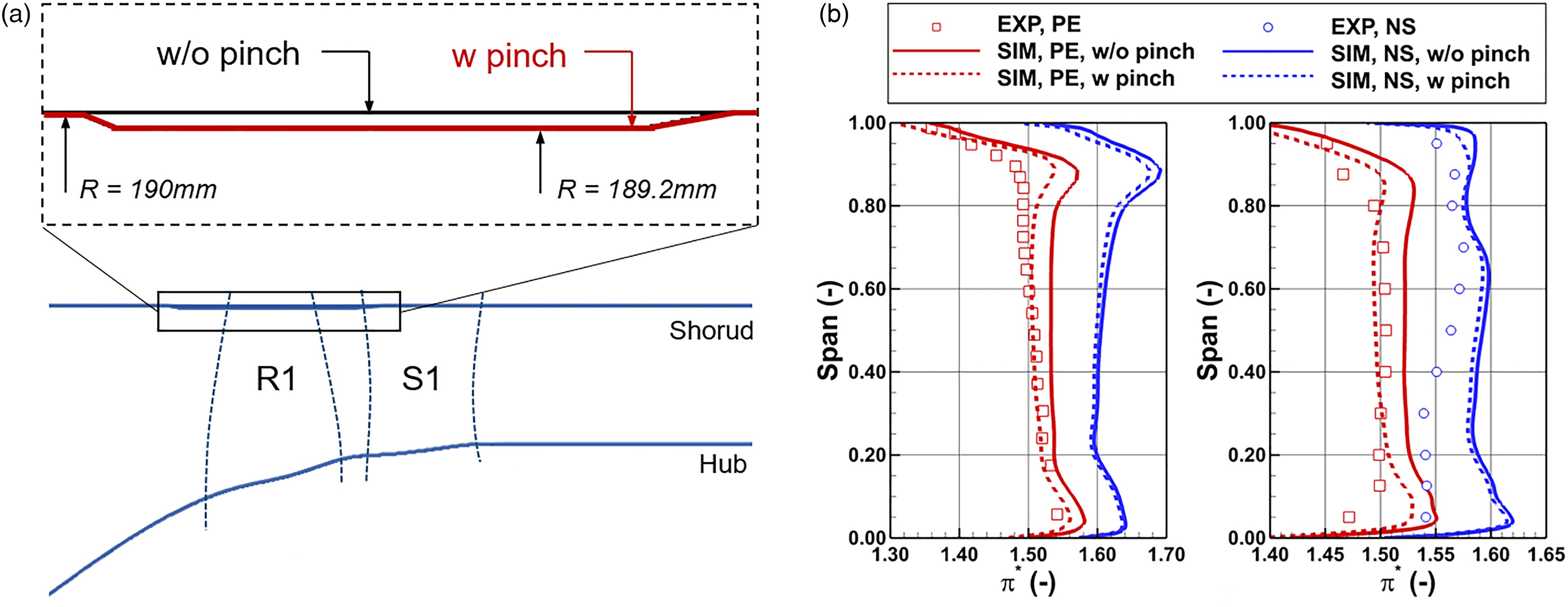
Effect of rotor casing pinch

In the experiment, a small pinch exists on the rotor casing endwall, but it is simplified as a smooth straight line in previous simulations. The shape of the pinch is illustrated in Figure 15a. In this section, the compressor with the realistic pinched casing is simulated by using the CFX solver, the Fine grid, the SST turbulence model and the mixing plane rotor-stator interface model. The radial profiles of the total pressure ratio are presented in Figure 15b. In general, the rotor casing pinch reduces the total pressure ratio at all spans, which improves the agreement with the measured data. This is because the pinched casing reduces the rotor throat area, increases the axial velocity (when comparing at the same mass flow), reduces the work input (by changing the rotor exit velocity triangle) and eventually reduces the total pressure ratio. Such a reduction effect is more evident in the PE condition than in the NS condition, because the slope of the total pressure ratio characteristic is steeper near the PE condition.

Figure 15.

Effect of rotor casing pinch. (a) Illustration of rotor casing pinch (b) Radial profiles at the rotor exit (left) and the stage exit (right).

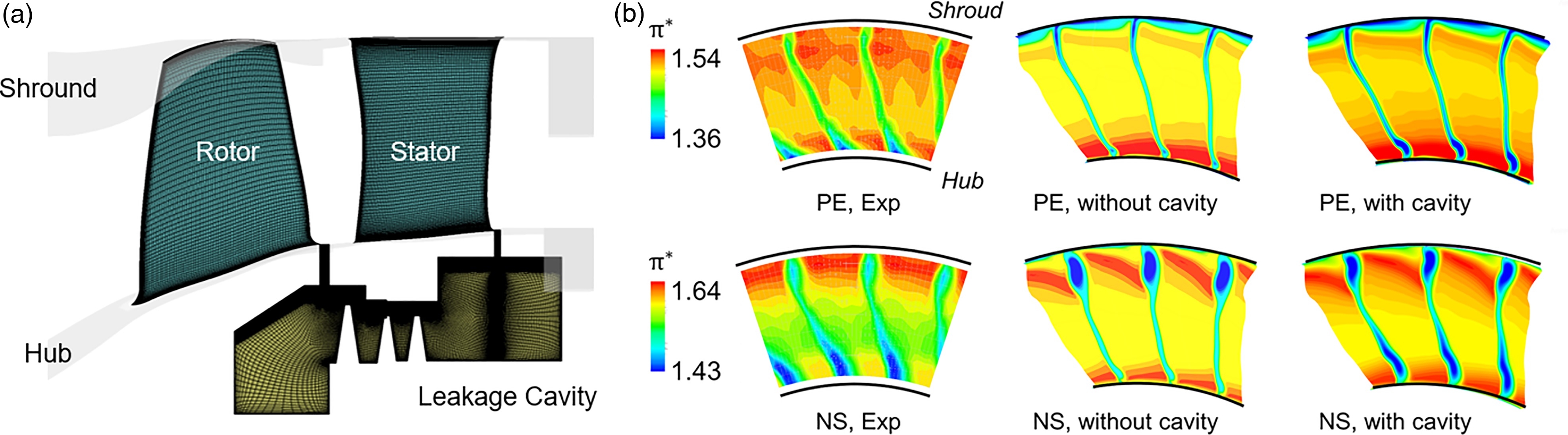
Effect of stator hub cavity

In the test rig, a secondary flow passage connects the stator inlet hub to the stator outlet hub, and a leakage flow may exist. To explore its effect on the prediction, a cavity geometry shown in Figure 16a is investigated numerically in this section. The simulation is conducted using the CFX solver, the Fine grid, the SST turbulence model and the mixing plane rotor-stator interface model. The total pressure ratio contours at the stage exit (ME30) are presented in Figure 16b. It shows that the stator hub cavity increases the near-hub total pressure loss at both the PE and the NS conditions, leading to slightly better agreement with the measured data. However, because the leakage mass flow rate of the investigated cavity geometry is only about 0.2% of the main flow rate, its effect is not strong enough to eliminate the near-hub disagreement with the measured data. According to previous research (Seshadri et al., 2015), a leakage mass flow rate of about 0.5% can potentially help match the measured data better. A parametric study of the cavity leakage flow rate will be pursued for future research.

Figure 16.

Effect of stator hub cavity. (a) Illustration of stator hub cavity (b) Total pressure ratio contours at the stage exit (ME30).