Introduction

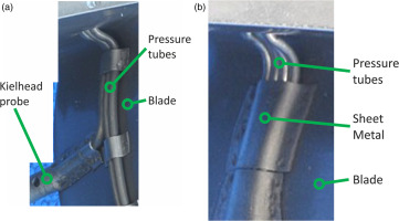
Although more accurate numerical models are increasingly used in numerical flow simulation due to decreasing computational costs in the last decades, experimental tests on multistage compressor rigs are still necessary to validate the numerical predictions. In order to measure quantities such as total temperature or total pressure within the rig, Kielhead probes, which are attached to the leading edges of the stators, are often used (see Figure 1a). The static profile pressure distribution on the surfaces of the stator blades is measured by static pressure taps. In particular, it is in the rear stages of the compressor that the tubes connecting the probes or the taps to the measuring devices outside the rig cannot be routed inside the blade for structural strength reasons. Instead, the tubes are attached to the blade surface and sometimes covered with a thin sheet of metal (see Figure 1b). This inevitably leads to considerable changes in the blade geometry since the dimensions of the pressure tubes can be in the same order of magnitude as the blade thickness. As a result, this produces additional total pressure losses, which ultimately affect the measured efficiency of the rig. This efficiency deviates from the numerically calculated efficiency of a non-instrumented rig due to the effects of the intrusive measurement technique and so must subsequently be corrected to take this error into account.

Figure 1.

Pressure tubes on the surface of an axial compressor blade. (a) Connecting Kielhead probes. (b) Connecting static profile pressure taps.
https://journal.gpps.global/f/fulltexts/192450/JGPPS-00215-2023-01.01_min.jpg

The literature on this subject provides a number of insights into the effects of these pressure tubes when mounted on the surface of compressor and turbine blades. Most studies, however, have investigated pressure tubes in combination with airfoil probes at the stator leading edge, which makes separating the effects of these two blade modifications challenging. Ma and Jin (2016) conducted numerical and experimental tests on the effects of two airfoil probes with spanwise pressure tubes at various span- and chordwise positions on the pressure side of a compressor blade. All tests were conducted at low Reynolds and Mach numbers of 150,000 and 0.05 respectively. For the case which is most comparable to the setup we examined (case 348), they reported that the integral total pressure loss coefficient increased by approximately 90% when a pressure tube was placed at 30% of the chord length and two airfoil probes were added at 45% and 85% spanwise height. Although Ma and Jin did not specify the amount of total pressure loss generated by the tubes and probes individually, their data shows that wake regions unaffected by the two airfoil probes still exhibited an increased total pressure loss of approx. 60%. In a follow-up paper to this study, Ma et al. (2017) conducted additional RANS simulations at a higher Mach number of 0.7. The results showed that the flow on the pressure side separates from the blade surface upstream of the spanwise pressure tubes and subsequently reattaches downstream. The distance between the upstream separation and the pressure tube is approx. four times the pressure tube diameter while the distance between the pressure tube and the reattachment line is approx. 18 times the pressure tube diameter. A similar separation behavior was reported by Zhang et al. (2023), who added three airfoil probes (5% span, 50% span and 95% span) to the leading edge and a spanwise pressure tube at 50% chord length to the compressor cascade blade V103-220. This phenomenon contributes to an overall increase in the total pressure loss coefficient by approx. 20%. Compared to the total pressure loss increase reported by Ma and Jin (2016), this loss increase is moderate and results from the fact that a spanwise pressure tube is less critical when placed closer towards the trailing edge. It is not clear, however, in the study by Zhang et al. (2023) how much of this total pressure coefficient increase can be attributed to the presence of the spanwise pressure tubes, since the interaction of the vortices induced by the airfoil probe with the separated regions and the corner vortices is highly complex.

As far as we know, only Chernoray et al. (2010), and Lalit et al. (2010) examined the effects of spanwise bumps on the suction and pressure side of turbine blades as part of their work on surface non-conformances caused by welding traces. The size of the surface non-conformance investigated was chosen as being 20% of the blade maximum thickness, which is smaller than the pressure tubes examined in our study, but still in the same order of magnitude. Chernoray et al. (2010) found that whenever such a surface non-conformance was placed on the suction side, a large open recirculation zone was formed. They identified the location of the welding trace at 20% chord length to be the most critical with an increase in the total pressure loss coefficient by a factor of almost ten. When placed at 30% chord length, the losses still increased by a factor of three. The pressure side proved to be insensitive towards any placement of a welding trace there. The authors also compared their experimental data to numerical RANS simulations and showed that only the kω-SST model was able to reproduce the general trends in the data with reasonable accuracy. On the other hand, the kϵ model failed to predict the total pressure loss increase completely. In the profile pressure data published by Lalit et al. (2010) for the same setup, it can be seen that the effects of such a surface non-conformance is significantly more pronounced when found in a region of adverse pressure gradient. When placed close to the leading edge, the flow is able to reattach to the suction side, having almost no effect on the overall vane loss. Lalit et al. (2010) also found that the additional flow losses are in fact profile losses. Losses generated by the sidewalls and corner regions were not changed by the presence of the welding trace.

As this review of the existing literature shows, to date, there are no studies that consider the effects of spanwise pressure tubes on the surface of compressor blades in isolation. For the investigations described in this paper, we chose a particularly critical case, which arises when the tubes are mounted on the pressure or suction side of a blade of a rear high-pressure compressor stage. These modified blades were investigated experimentally in the linear cascade wind tunnel of the Institute of Jet Propulsion and Turbomachinery (IST) at the RWTH Aachen University. Numerical RANS simulations were used to examine the experimental results in more depth.

Methodology

Modelling of the pressure tubes

For the purpose of this study, we modeled the pressure tubes covered by a sheet of metal as a simplified bump. This bump, modeled on a flat plate for clarity, is presented in Figure 2. The variables h and w denote the height and width of the bump, respectively, while r1 and r2 represent the radii. The radii r1 and r2 have been chosen so that all transitions of the bump boundary curve are tangential. The flat plate bump geometry is then scaled appropriately and transferred onto the curved surfaces of the blade (see Figure 3). These bumps extend across the full span of the blade with a width of 24% of the chord length and a height of 67% of the maximum blade thickness. The leading edge of the bumps is located at 30% of the streamwise surface length. All cascade blades have a fillet at the blade root and tip to dampen the formation of the corner vortex and maintain a two-dimensional flow over a large midspan region. When the bump is applied to the pressure side, we call this “pressure-sided bump” (PSB) and when added to the suction side, “suction-sided bump” (SSB).

Figure 2.

Simplified pressure tube geometry.

https://journal.gpps.global/f/fulltexts/192450/JGPPS-00215-2023-01.02_min.jpg
Figure 3.

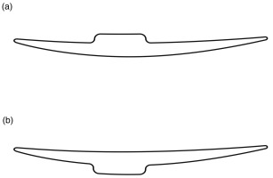
Compressor blade with pressure tubes. (a) On the pressure side. (b) On the suction side.

https://journal.gpps.global/f/fulltexts/192450/JGPPS-00215-2023-01.03_min.jpg

Experimental setup

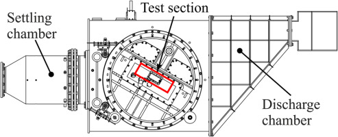
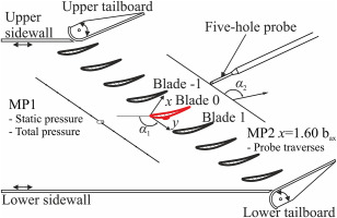
A high subsonic compressor cascade profile, which has already been used in previous investigations of our institute (Winter et al., 2013), was selected. The experiments were conducted at the linear cascade wind tunnel of the institute (see Figure 4). The air is supplied by a multistage radial compressor, which enables experiments in a Mach number range of 0.4 up to 0.85. Due to the closed-loop design, an engine-like Reynolds number between 650,000 and 1,250,000 can be adjusted independently of the Mach number. For the profile we selected, an inlet Mach number of about Ma0.5 and an isentropic Reynolds number of Re=790,000 were chosen as the operating point. Before entering the test section, the flow is homogenized and the turbulence is reduced in the settling chamber using honeycomb screens. With a passive turbulence grid located in the settling chamber, a turbulence level of approximately 2.5% is generated directly upstream of the blades. The flow is accelerated by a convergent nozzle and enters the rectangular cross section of the test section where the compressor cascade, consisting of nine blades, is located (see Figure 5). Adjustment of the operating point is achieved by measuring the total pressure in Measuring Plane 1 (MP1) with a pitot-probe and using static wall pressure taps. Measurements downstream of the three central blades (labeled as Blade −1, 0, 1 in Figure 5) were performed at midspan of the blade with a five-hole probe. The wake measurements were made at 60% of the axial chord length bax downstream of the trailing edge, referred to as Measuring Plane 2 (MP2), due to the occurrence of large separation bubbles, as will be shown later. Downstream of the test section, the discharge chamber is located.

Figure 4.

Linear cascade wind tunnel.

https://journal.gpps.global/f/fulltexts/192450/JGPPS-00215-2023-01.04_min.jpg
Figure 5.

Cascade test section with modified central blade (blade 0).

https://journal.gpps.global/f/fulltexts/192450/JGPPS-00215-2023-01.05_min.jpg

A cascade with only nominal blades is used as the reference case for this study. This configuration will be referred to as “clean blade” in the following. The periodicity of the flow is set for the clean blade cascade using the adjustable sidewalls and tailboards. To evaluate the influence of a spanwise bump, the central blade “Blade 0” is replaced by a modified blade with either a pressure-sided or a suction-sided bump, while all other blades remain nominal (see Figure 5). The additional losses generated by these bumps are found by comparing the modified cascade to the nominal cascade. The sidewall and the tailboard settings are not changed in relation to the clean blade cascade. All changes in the periodicity of the flow are therefore due to the influence of the bump. For the nominal cascade, only the wake of the central blade “Blade 0” is measured. In the case of the pressure-sided bump, the wake of the central modified blade is measured, while for the suction-sided bump, the pressure side-adjacent and suction side-adjacent blades (“Blade −1” and “Blade 1”) are measured as well. This configuration, in which there is only one modified blade surrounded by clean blades, is similar to a test rig which has only a few instrumented blades.

The profile loss is evaluated in terms of the local total pressure loss coefficient ω, which is defined as

(1)
ω=pt1pt2pt1ps1.

The total inlet pressure pt1 is measured using a pitot-probe and the static inlet pressure ps1 is measured using pressure taps in MP1. The total outlet pressure pt2 is determined by means of the five-hole probe in MP2 using a look1up table approach. The measurement uncertainty is determined with linear Gaussian error propagation, resulting in a maximum uncertainty value of Δω/ωmax,clean,exp=0.52%. This value is given in relation to the experimentally determined maximum value of the clean blade total pressure loss coefficient ωmax,clean,exp. To characterize the flow losses by a single value, the integral total pressure loss coefficient ωint is calculated by

(2)
ωint=pt1¯pt2¯pt1¯ps1¯.

Here, pt2¯ denotes the mass flow averaged total outlet pressure in MP2 while pt1¯ stands for the mass flow averaged total inlet pressure in MP1. In order to eliminate the free stream loss of the flow from MP1 to MP2, a correction is applied to pt1¯. The mean static pressure at MP1 is expressed by ps1¯. A Monte-Carlo analysis was used to determine the measurement uncertainty of ωint, resulting in a value of Δωint/ωint,clean,exp=2.68%.

Since the blade geometry investigated is proprietary, all data on the total pressure loss coefficient ω is normalized. In the plots, ω is normalized with respect to the experimentally determined maximum value of the local total pressure loss coefficient for the clean blade ωmax,clean,exp. Integral values of ω for both experimental and numerical results are normalized with respect to the integral total pressure loss coefficient of the clean blade ωint,clean. The coordinate in pitchwise direction y, which is plotted on the x-axis of all wake plots, is normalized by the blade pitch t.

Numerical setup

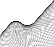
To simulate the effects of the spanwise pressure tubes on the flow around the compressor blade, we used the code TRACE 9.4 (Turbomachinery Research Aerodynamic Computational Environment), which is developed by the German Aerospace Center (DLR) in cooperation with MTU Aero Engines. We solved the RANS equations with a finite volume scheme of second-order spatial accuracy by applying a MUSCL approach together with a central discretization of the viscous terms and Roe upwind-based convective flux difference splitting. In this study, the kω turbulence model by Wilcox (Wilcox, 1988) and the SST model by Menter et al. (2003) were used. The stagnation point correction by Kato and Launder (1993) was applied to both models. The transition was modelled by the γReθ transition model by Menter et al. (2004) in the formulation from 2009 (Langtry and Menter, 2009) for both turbulence models. Additionally, we also conducted simulations using the kω model with activated Viscous Blending (VB) limiter, which limits the production of turbulent kinetic energy in the vicinity of the blade in order to improve the blade wake shape. Further details on this limiter can be found in the paper by Bode et al. (2014). All meshes were generated with AutoGrid 14.1 applying a structured meshing approach. Since the radii of the pressure tubes are comparatively small, a high mesh resolution was chosen to ensure a faithful reproduction of the smooth geometry by the mesh. A close-up of the mesh near the bump can be seen in Figure 6. For all models, the value of y+ was kept close to one to ensure an appropriate resolution of the boundary layer. All inlet boundary conditions were derived from experimental data acquired in MP1. The turbulent decay was adjusted via the specific turbulent dissipation rate so that the turbulent kinetic energy directly upstream of the leading edge matched the experimentally measured value.

Figure 6.

Close-up of the mesh near the bump.

https://journal.gpps.global/f/fulltexts/192450/JGPPS-00215-2023-01.06_min.jpg

Pressure-sided bump

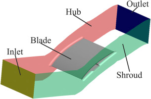
In order to achieve mesh independence for every turbulence model, multiple mesh refinement studies were conducted. In the case of the pressure-sided bump, a single-passage approach (see Figure 7) was chosen, since the influence of the pressure-sided bump is mostly limited to the flow around the modified blade itself. Approximately 29 million cells were sufficient for the pressure-sided bump to achieve mesh independence with regard to the integral total pressure loss coefficient ωint when the kω turbulence model was used (see Table 1, first column). For the SST turbulence model, it was not possible to achieve full mesh convergence even with a mesh of 53 million cells (see Table 1, second column). However, since a continuation of the mesh independence study with even finer meshes was not feasible due to limited computational resources, the mesh with 53 million cells was considered to have a sufficiently fine resolution. The results of the kω model with activated VB limiter were almost identical to those of the SST model.

Figure 7.

Single-passage domain for the pressure-sided bump.

https://journal.gpps.global/f/fulltexts/192450/JGPPS-00215-2023-01.07_min.jpg
Table 1.

Integral total pressure loss coefficients resulting from the mesh independence.

Pressure-sided bumpSuction-sided bump
Cells [*106]ωint/ωint,clean,expCells [*106]ωint,3/ωint,clean,exp,3
kωSSTkωSST
3.972.822.2735.064.653.84
22.122.771.8552.703.693.85
29.482.852.14
53.032.891.93

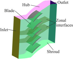
In the experiment performed, only the central blade of the cascade was modified, while all other blades were identical to the nominal blade. In the numerical simulations, however, this setup cannot be implemented due to the periodic boundary conditions in the pitch direction. A single-passage simulation here is equivalent to an infinite cascade where each blade is modified. In the case of large-scale flow separation, however, this approach is of limited value because the modified blade can influence the adjacent nominal blades. In order to verify whether there is influence from the neighboring blades and, if so, how large their influence is, simulations containing several passages were performed. In these multi-passage simulations, periodic boundary conditions were still used, but only the central blade was modified, so that the numerical model is equivalent to an infinite cascade in which only every n-th blade is modified. Since the adjacent nominal blades could be resolved using a much coarser mesh, they were connected to the mesh of the modified blade via non-matching zonal interfaces (see Figure 8 for the five-passage model).

Figure 8.

Five-passage domain for the suction-sided bump.

https://journal.gpps.global/f/fulltexts/192450/JGPPS-00215-2023-01.08_min.jpg

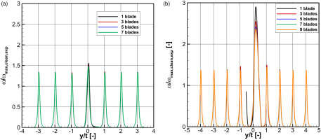
For the pressure-sided bump, four setups were investigated using 1, 3, 5 and 7 blades respectively. In these setups, only the central blade was modified. Figure 9a shows the resulting total pressure loss coefficient distribution in MP2, normalized by ωmax,exp,clean. The analysis of ωint of the central blade revealed that the single-passage model deviates less than 0.01 in relation to the seven-passage model for both the kω model and the SST model (see Table 2). Therefore, the single-passage model was considered appropriate for the investigation of the pressure-sided bump. By comparing the y/t-coordinate of the total pressure loss coefficient maxima, the changes in the flow turning depending on the number of passages can be seen. If only one passage is included in the numerical model, the resulting wake exhibits less flow turning than the models with 3, 5 or 7 passages. When comparing these multi-passage models, no significant difference can be found. This deviation in the flow turning by the single-passage model is a drawback. However, since we are mainly interested in the losses generated by the bump, this deviation is considered to be acceptable when considering the computation time.

Figure 9.

Total pressure loss coefficients in MP2 for a varying number of blades, calculated with the kω turbulence model. (a) Pressure-sided bump. (b) Suction-sided bump.

https://journal.gpps.global/f/fulltexts/192450/JGPPS-00215-2023-01.09_min.jpg
Table 2.

Integral total pressure loss coefficient for varying number of simulated blades.

Pressure-sided bumpSuction-sided bump
Bladesωint/ωint,clean,expBladesωint,3/ωint,clean,exp,3
kωSSTkωSST
12.771.8533.874.25
32.741.8153.693.85
52.741.8473.653.89
72.741.8593.663.88

Suction-sided bump

For the suction-sided bump, the mesh independence study was conducted with a domain consisting of five blades to account for the effects of the suction-sided bump on the adjacent blades. For the same reason, in the case of the suction-sided bump, the integral pressure loss coefficient ωint,3 is always given for the central three blades. The mesh was only refined in the central passage. For both the kω model and the SST model, mesh independence was achieved at approximately 52.7 million cells (see Table 1, third and fourth column). None of the simulations using the kω model with activated VB limiter converged.

In order to check how many blades have to be included in the numerical domain to capture the effects of the adjacent nominal blades, we simulated models with 1, 3, 5, 7 and 9 blades respectively. The domain containing five blades is shown in Figure 8) as an example. In Figure 9b, the corresponding normalized total pressure loss coefficient distributions are shown. This plot clearly demonstrates, that the result of the setup with one blade only differs significantly from all other simulations, which is why this setup was not considered appropriate for this case. What is also evident is that the suction-sided bump influences not only the losses generated by the central blade, but those of the adjacent blades too. For the suction-sided pressure tubes therefore, we integrated the total pressure loss over the central three blades. We found that by simulating five blades, the integral total pressure loss coefficient deviated by 0.03 from the model with nine blades for both turbulence models. This deviation is in the same order of magnitude as the measurement uncertainty. The data can be found in Table 2, normalized by the experimental value for the integral total pressure loss coefficient of the central three blades of an unmodified cascadeωint,clean,exp,3. Since the setup with 9 blades increased the cell count by 64% compared to the setup with 5 blades, the latter was deemed more appropriate given the required computation time.

Results and discussion

Clean blade

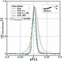
Before discussing the results of the modified blades, we first evaluate the performance of the CFD solver in the case of the clean blade by comparing the local and the integral total pressure loss coefficient to the experimental data. Figure 10 shows the normalized local total pressure loss coefficient for the experiment as well as the simulation results using the kω turbulence model both with and without VB limiter and the SST turbulence model for one pitch. All wakes were centered with regard to the experimentally determined wake center, which makes it easier to identify the shift in the turning of the flow. The kω model with activated VB limiter as well as the SST model are able to predict the shape of the wake flanks with very good accuracy. The peak value is overpredicted by ca. 35%. The simulation without VB limiter predicts the wake as being much wider than the experimental data due to an overproduction of turbulent kinetic energy around the blade. This overproduction leads to a wrong prediction of the transition location on the suction side, which is now located close to the leading edge, resulting essentially in a fully turbulent flow around the blade. The overestimation of the peak is similar to that simulated by the activated VB limiter. Table 3 indicates the integral pressure loss coefficients, normalized relative to the value of the experimental data of the clean blade. The setups with the kω model and VB limiter as well as the SST model are able to reproduce the experimental value with deviations of 0.1 and 0.07, respectively. Without the VB limiter, the larger wake leads to a 1.85 times larger integral total pressure loss coefficient compared to the experimental value.

Figure 10.

Comparison of experimental data for the clean blade with results from numerical simulations using the kω turbulence model both with and without VB limiter and the SST model.

https://journal.gpps.global/f/fulltexts/192450/JGPPS-00215-2023-01.10_min.jpg
Table 3.

Normalized integral total pressure loss coefficient of the clean blade.

ωint,clean/ωint,clean,exp
Experiment1.00
CFD kω model1.85
CFD kω model VB1.10
CFD SST model1.07

Pressure-sided bump

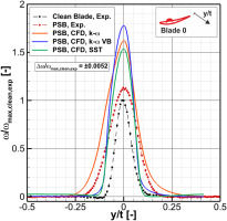
To evaluate the additional total pressure losses caused by the pressure-sided bump, we investigated the total pressure loss coefficient in the wake of the modified blade. As the CFD results indicate that most of the additional total pressure losses are generated in the wake of the modified blade, the wakes of the adjacent blades have not been investigated further in this study. To improve the comparability of the wakes and to eliminate the influence of the single-passage model on the flow turning, all wakes were centered with regard to their loss maxima. Figure 11 shows the experimental local total pressure loss coefficient for both the modified and the clean blade, as well as the numerical results of a single-passage simulation with a pressure-sided bump for the different turbulence model settings mentioned previously. When comparing the two experimental data, we find that the wake of the modified blade is wider than that of the clean blade and the peak is approx. 12% higher. By calculating the integral total pressure loss coefficient, we can observe that the PSB leads to an increase in ωint by a factor of 1.9 in the experiment by widening the wake (see Table 4).

Figure 11.

Total pressure loss coefficient for the PSB blade.

https://journal.gpps.global/f/fulltexts/192450/JGPPS-00215-2023-01.11_min.jpg
Table 4.

Normalized integral total pressure loss coefficient of the PSB blade.

ωint/ωint,cleanωint/ωint,PSB,exp
Experiment1.901.00
CFD kω model1.541.50
CFD kω model VB1.811.04
CFD SST model1.771.02

[i] *Corresponding integral total pressure loss coefficient of the clean blade for the experiment/each turbulence model.

The kω model, regardless of the VB limiter and the SST model overpredict the maximum local total pressure loss coefficient. Without activated VB limiter, the wake predicted by the kω model is too wide on both the suction side and pressure side. Again, like the in the case of the clean blade (see Figure 10), this setup leads to an overproduction of turbulent kinetic energy, which results in a fully turbulent boundary layer on the suction side. This, together with the overproduction of turbulent kinetic energy on the pressure side, leads to a wake which is much wider than measured in the experiment. For the kω model with activated VB limiter and the SST model, the transition on the suction side is correctly simulated and therefore the right wake flank matches the experimental data better. As a result, the setup “kω model” overpredicts ωint by 1.5 (see Table 4, second column). Using both the kω model with activated VB limiter and the SST model, ωint, normalized with regard to the experimental value, is calculated much more accurately with a value of 1.04 and 1.02, respectively (see Table 4, second column). When comparing the wakes calculated with kω VB and SST to their corresponding “clean” wakes in Figure 10, a clear widening of the wake especially at the left flank, which is associated with the pressure-sided bump, can be observed. In order to evaluate the performance of the turbulence models further, we normalized each integral total pressure loss coefficient by the corresponding integral total pressure loss coefficient of the clean blade for each turbulence model (see Table 4, first column). This analysis shows that the kω model with VB limiter and the SST model are able to closely match the trend shown by the experimental data. The kω model, however, predicts a loss increase of only 1.54 times the loss of the clean blade also simulated with the kω model. This is a result of the integral loss calculated by this model for the clean blade already being much larger than for the other turbulence models.

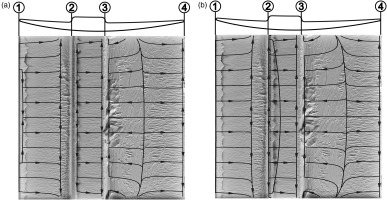
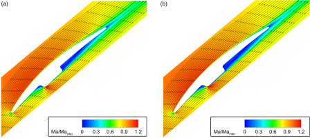
Using surface oil flow visualization, we further analyzed the flow distortions caused by the PSB on the surface of the pressure side. The resulting oil flow pattern was then compared to the numerically obtained wall stream lines for the kω model (see Figure 12a) and for the SST model (see Figure 12b). The wall stream lines for the kω model with VB were basically identical to those of the SST model and are therefore not shown here. Early transition via a separation bubble is evident from the accumulation of paint near the leading edge, followed by a coarse streamline pattern due to turbulent flow. The same flow behavior was observed for the clean blade near the leading edge by Hoesgen (2019), who conducted surface hot-film measurements, as well as oil flow visualization. Upstream of the rising flank of the bump, the flow detaches again, forming a separation bubble. The flow then reattaches on top of the bump. This flow behavior is similar to the flow over a forward-facing step. At the falling flank of the bump, the flow once again detaches and then reattaches downstream on the pressure side, forming a closed separation bubble. The formation of a closed bubble is favored by the concave surface of the pressure side. The lines perpendicular to the flow direction, which are visible downstream of the bump, are caused by the application of the paint with brush strokes in this direction. In this area, the paint did not follow the flow because the velocity in the separation bubble was too low. This flow behavior is correctly reproduced by all numerical setups used, which is illustrated by the overlying wall stream lines in Figure 12. Compared to the kω model, the SST model predicts a slightly larger separation bubble on top of the bump. Apart from this, both numerical results are in good agreement with the oil flow visualization, considering the rather qualitative nature of oil flow visualization. One further insight is given by the Mach number distribution in the midspan of the PSB blade normalized by the inlet Mach number in Figure 13. The previously described separation upstream, and downstream as well as on top of the bump, are visible.

Figure 12.

Oil flow visualization with overlaid wall streamlines for the PSB blade. ①: leading edge, ②: rising flank, ③: falling flank, ④: trailing edge. (a) Wall streamlines of kω model. (b) Wall streamlines of SST model.

https://journal.gpps.global/f/fulltexts/192450/JGPPS-00215-2023-01.12_min.jpg
Figure 13.

Normalized Mach number distribution in midspan of the PSB blade. (a) kω model. (b) SST model.

https://journal.gpps.global/f/fulltexts/192450/JGPPS-00215-2023-01.13_min.jpg

In conclusion, the numerical simulations are able to capture the trends of the experiments quite well. All turbulence models lead to a considerable increase in the integral total pressure loss coefficient, ranging from an increase by a factor of 1.54 to 1.81 caused by the PSB. The comparison between the oil flow visualizations and the numerically determined wall stream lines further demonstrates that the general flow physics is satisfactorily reproduced. Only the local distributions of ω reveal the weaknesses of the numerical simulations as they are unable to match the experimental distribution. This is to be expected however, since RANS models rarely perform well for flow cases with large separations. Overall, this study demonstrates that a PSB has a significant effect on the losses generated by a blade and that this effect can be reproduced with RANS simulations by application of a single-passage model.

Suction-sided bump

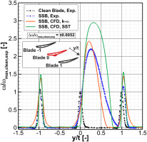
Analogous to the pressure-sided bump, Figure 14 shows the local total pressure loss coefficient for the blade modified with a suction-sided bump (SSB) and the clean blade for both the experimental and numerical results. As previously discussed, a domain with five blades was used to simulate the flow. As the SSB only significantly influences the losses generated in the central three passages, those results are shown in Figure 14. Again, all wakes were centered with regard to the experimentally determined wake center. The kω model with VB limiter did not converge for the suction-sided bump and is therefore not shown.

Figure 14.

Total pressure loss coefficient of the SSB blade.

https://journal.gpps.global/f/fulltexts/192450/JGPPS-00215-2023-01.14_min.jpg

From Figure 14, it is immediately apparent that the losses caused by the SSB are much larger than those caused by the PSB. Compared to the clean blade, the peak value of the suction-sided bump is 2.2 times larger. The flow deflection is reduced, as shown by the positive y-shift of the wake. Furthermore, the wake is much wider and extends into the wake of the adjacent blade, which can be seen by the fact that ω does not reach the freestream loss level of close to zero at y/t=0.9, resulting in the merging of both wakes. This once again confirms that a single-passage numerical model is not sufficient for the suction-sided bump. In the wake of the suction side-adjacent blade, additional losses are generated as indicated by a higher peak value of 15% and a wider wake compared to the clean blade. This is caused by a local positive incidence in the inflow of this blade due to the bump blocking the passage and the associated redistribution of the mass flow. Compared to the clean blade, the flow deflection is reduced. The influence on the wake adjacent to the pressure side is negligible. To account for the influence of the suction-sided bump on the adjacent blades, the integral loss coefficient is calculated for three wakes. The suction-sided bump increases the loss of the three blades by a factor of 4.10, as given in the first column of Table 5.

Table 5.

Normalized integral total pressure loss coefficient of the SSB blade.

ωint,3/ωint,clean,3ωint,3/ωint,SSB,exp,3
Experiment4.101.00
CFD kω model1.970.90
CFD SST model3.550.94

[i] *Corresponding integral total pressure loss coefficient of the clean blade for the experiment/each turbulence model.

As seen for the pressure-sided bump, both the kω model and the SST model overpredict the maximum local total pressure loss coefficient. Again, the kω model manages to predict the left side of the wake more effective than the SST model, which shows better agreement with the right side of the wake. In contrast to the experimental data, both models predict that the wake reaches the freestream loss level. According to the kω model, this is the case at y/t=0.65 whereas the wake of the SST model is wider and reaches the freestream level at y/t=0.8 and thus closer to the experiment. For the adjacent blades, the SST model performs significantly better than the kω model since it is better able to predict the losses of the clean blade. A further difference is the prediction of the turning of the flow, which is underestimated by the kω model whereas the SST model shows an overprediction. As both turbulence models predict a smaller wake compared to the experimental data, they both underestimate the increase in the integral total pressure loss coefficient ωint,3. The SST model performs slightly better than the kω model by deviating only 6% from the experimental value instead of 10%. Like for the PSB blade, we can normalize ωint,3 with the corresponding value for each turbulence model for the clean blade. This will enable us to assess whether the turbulence models can predict the relative loss increase correctly (see Table 5, first column). From this evaluation, we conclude that the SST model underpredicts the loss increase with a factor of 3.55 compared to the experiment (factor of 4.10). The relatively poor agreement with the experiment, that is a loss increase of only a factor of 1.97 for the kω model, is mainly due to the higher clean blade loss when the VB limiter is not being used (see Table 3).

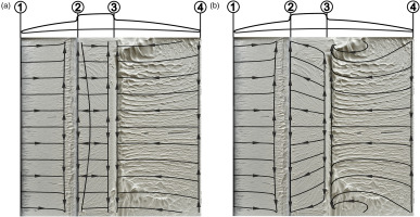
To analyze the reason for the large difference between the two models and to quantify which of these describes the flow physics more accurately, we again performed an oil flow visualization. The results for the suction side with the bump are depicted in Figure 15, with overlaid wall streamlines for both turbulence models. On the suction side, there is no transition with a laminar separation bubble at the leading edge due to a favorable pressure gradient. Hoesgen (2019) determined that the transition occurs between 30% and 50% of the axial chord length, which in this case coincides with the location of the bump. The separation bubble upstream of the bump therefore triggers the transition from laminar to turbulent. At the top of the bump, the streamlines are curved toward the midspan and are not parallel to the inflow and the channel walls. Downstream of the bump, the backward-facing step again causes a separation bubble. Unlike for the pressure-sided bump, there is no reattachment line, indicating a fully separated flow with an open separation bubble extending beyond the trailing edge. In the vicinity of the bump, large amounts of paint accumulate near the cascade walls.

Figure 15.

Oil flow visualization with overlaid wall streamlines for the SSB blade. ①: leading edge, ②: rising flank, ③: falling flank, ④: trailing edge. (a) Wall streamlines of kω model. (b) Wall streamlines of SST model.

https://journal.gpps.global/f/fulltexts/192450/JGPPS-00215-2023-01.15_min.jpg

The area upstream of the bump is predicted similarly by both models, correctly predicting the separation bubble at the forward-facing step. However, the results for the surface of the bump and downstream of the bump differ significantly. A small closed separation bubble is present for the kω model, resulting in a reattached flow on the bump surface with inflow parallel streamlines. In contrast, the SST model shows that the flow does not reattach at the bump surface, as indicated by the curved wall streamlines which are similar to the oil flow streamlines. While both models predict a fully separated flow downstream of the bump, the SST model exhibits two vortices that correspond to the accumulation of paint near the cascade walls. In these two areas, paint accumulates and is then entrained by the flow and carried away from the blade surface. In conclusion, this oil flow visualization shows that the occurring flow phenomena are much more effectively modeled by the SST model. The results of the kω model can be regared as physically incorrect.

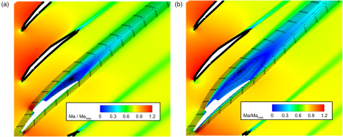
The difference between the kω model and the SST model can again be seen by comparing the Mach number distribution in the blade midspan as presented in Figure 16. The wake and the separation bubble are smaller for the kω model because the flow reattaches at the bump surface, whereas for the SST model the separation at the beginning of the bump merges with the separation downstream of the bump to form a large separation bubble. This results in a wider wake, as indicated by the local total pressure loss coefficient in Figure 14. Due to the larger separation bubble, the turning of the flow is lower, resulting in the shift of the wake in a positive y-direction.

Figure 16.

Normalized Mach number distribution in midspan of the SSB blade. (a) kω model. (b) SST model.

https://journal.gpps.global/f/fulltexts/192450/JGPPS-00215-2023-01.16_min.jpg

Overall, these experiments show that the addition of a bump to the suction side of a blade leads to an increase in the total pressure loss of factor 4.1 over three passages. This drastic increase is only reproduced by the SST turbulence model, which is likewise the only model able to simulate the detached flow over the bump correctly. Considering the challenging flow physics present in this case, the numerical simulation is able to reproduce the experimental results with good accuracy.

Conclusion

In this paper, we presented an experimental and numerical evaluation of the influence of pressure tubes on the pressure and suction side of a compressor stator blade. We modelled the pressure tube geometry as a simplified bump mounted on the blade surface. When a bump was placed on the pressure side, the integral total pressure loss was increased by a factor of 1.9. All three turbulence models (kω, kω with VB limiter, SST) were able to reproduce this effect with reasonable accuracy. Oil flow visualizations showed the formation of a closed separation bubble on top of the bump as well as downstream on the pressure side of the blade. It was also possible to capture both of these flow phenomena by means of the numerical simulations. When placed on the suction side, the bump had an even larger effect. This affected not only the wake of the modified blade itself, but also the wake of the blade adjacent to the suction side, leading to a loss increase of factor 4.1 over three pitches. This considerable loss increase was caused by a large, open recirculation zone which formed as a result of the flow separation on the upstream flank of the bump, as demonstrated by oil flow visualization. For this case, only the SST turbulence model was able to capture the flow separation accurately and was therefore the only model which was able to reproduce the total pressure loss increase with reasonable accuracy. The kω model calculated a reattachment of the flow on top of the bump, which could not be confirmed by the experiment. In conclusion, we demonstrated that pressure tubes should preferably be placed on the pressure side of a compressor blade, whenever possible.

In practice, this study shows that the presence of such pressure tubes can alter the measurement data of both the Kielhead probes and the static profile pressure taps. The latter are expected to be highly sensitive to even minor changes in the flow field. As a result, the measured profile pressure distribution is likely to differ from the pressure distribution of a clean blade. In future work, we plan to integrate static pressure taps into the modified blades to measure the altered pressure distribution. Furthermore, we will investigate different pressure tube configurations by varying the geometrical dimension of the bump.

Nomenclature

ω

Total pressure loss coefficient (−)

ωint

Integral total pressure loss coefficient (−)

bax

Axial chord length (mm)

Ma

Mach number (−)

ps

Static pressure (Pa)

pt

Total pressure (Pa)

Re

Reynolds number (−)

t

Pitch (mm)

y

Pitchwise coordinate (mm)

IST

Institute of Jet Propulsion and Turbomachinery

MP

Measuring plane

PSB

Pressure-sided bump

SSB

Suction-sided bump

VB

Viscous Blending