Introduction

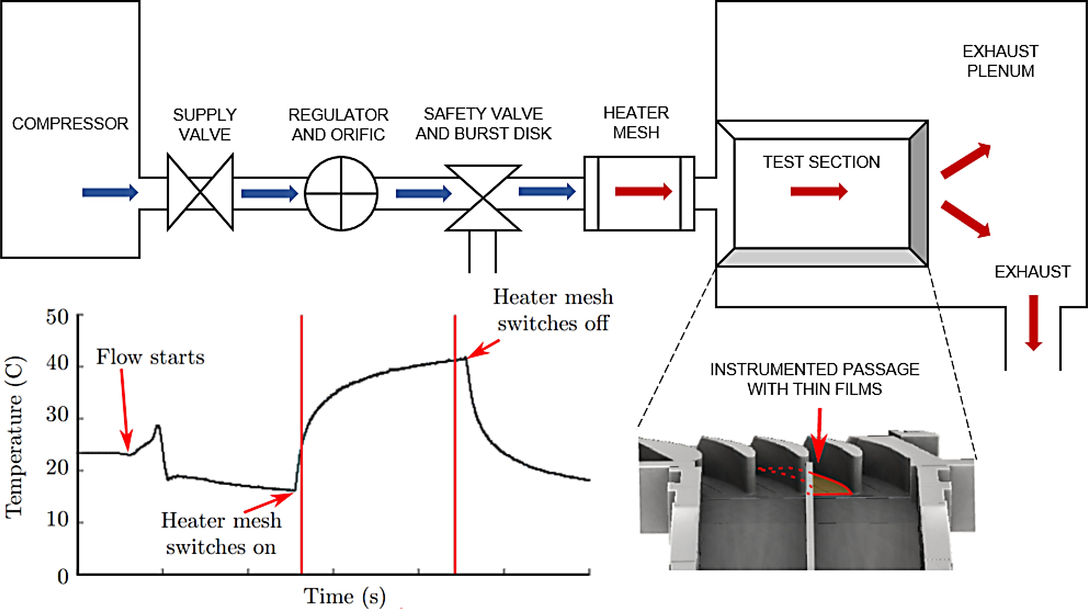
High speed linear cascades are often used to analyse aerodynamic performance of turbine blades, nozzle guide vanes and cooling systems. Compressed air is passed through a heater mesh to achieve near uniform step change in temperature across the operational section. Shown in Figure 1, the heated air is passed through the test cascade, optionally with cooling flow, to conduct heat transfer measurements. Alongside standard cascade measurements, thin films are adhered to the test section to allow high speed surface temperature measurement, without impeding design form or profile. The data is routinely post-processed using the impulse response method. A known temperature and heat flux signal, commonly the unit step solution, is used to derive a signal filter for heat flux. This filter is then applied to the measured temperature data to infer the surface heat flux in the test cascade.

Figure 1.

Example high speed linear cascade facility instrumented with thin film gauges on the passage endwall, with typical temperature measurement showing the used data window for heat flux calculation Shaikh (2020).

The derivation of the basis functions, used to construct the filter, assumes linear time invariance, uniform isotropic materials and surface normal heat transfer. These assumptions lead to limitations in the impulse response method, primarily the semi-infinite limit which caps the permitted test duration by the time for heat penetration through the material. The Schultz-Jones limit is commonly used, corresponding to a less than 1% back surface to front surface heat flux ratio Schultz and Jones (1973). This limit is a useful guide but is only valid in the case of uniform materials, planar surfaces, normal heat transfer and unit step heat flux. Care should be taken when applying this limit to convection tests on free-form geometry, when none of these underlying assumptions hold.

In contrast, numerical methods can handle much longer duration tests and, provided a back boundary condition is known, can post-process data beyond the semi-infinite limit. This does however necessitate the measurement of the back surface, often not accessible in many cascade designs. In the case of nozzle guide vane analysis, the “back surface” is considered the camber line of the vane due to heat penetration from both the pressure and suction surfaces.

Heat transfer test articles are often assemblies including laminates, parts or insulation with differing material properties. Traditional response methods assume a uniform isotropic material and thus do not accurately model these systems. The errors caused by this assumption are evaluated, along with the modifications necessary to accurately use the impulse response in multilayer analysis. An analytic solution and a new numerical method are both investigated to solve and validate the laminate problem. Both solution methods are demonstrated in the case of evaluating heat flux in thin film laboratory analysis.

1D multilayer analytic methodology

A variety of methods exist to analyse 1D transient heat transfer. The analytic derivation for several cases can be found in the Conduction of Heat in Solids by Carslaw and Jaeger (1947). Electrical analogies and thermal network models are commonly employed to approximate the material behaviour Shafaq et al. (2016). The Cook and Felderman (1966) piecewise linear approximation algorithm has been widely used. Improvements in computing hardware has seen a rise in both explicit and implicit numerical methods Walker and Scott (1998), Recktenwald (2011), and Bertolazzi et al. (2012) evaluated the use of finite elements. Oldfield (2008) presented a fast fourier transform implementation of the impulse response method, which is extensively used at the Oxford Thermofluids Institute (OTI). All of these methods have been demonstrated in the case of single and two layer analysis, but few have been stretched to the case of complex multilayer laminates.

Doorly and Oldfield (1987) showed that for long duration tests, when heat penetrates to the back substrate, a laminate construction has a significantly different behaviour to the single material case. To account for this, Oldfield (2008) published the analytic solution for a two-layer laminate with a simple kapton thin film and metal test section. His dual layer analytic solution for surface temperature has a more complicated basis function and many users choose to ignore this effect to simplify the analysis. Typically a single layer approximation is used, building the response functions with the material properties of the test geometry only, ignoring the thin film. It is common to select test materials with very low thermal diffusivity to impede heat flow into the material, thus increasing the time for heat penetration to the back surface, allowing a longer duration test. The bulk properties are thus similar to that of the thin film, and forms the justification for the single layer simplification.

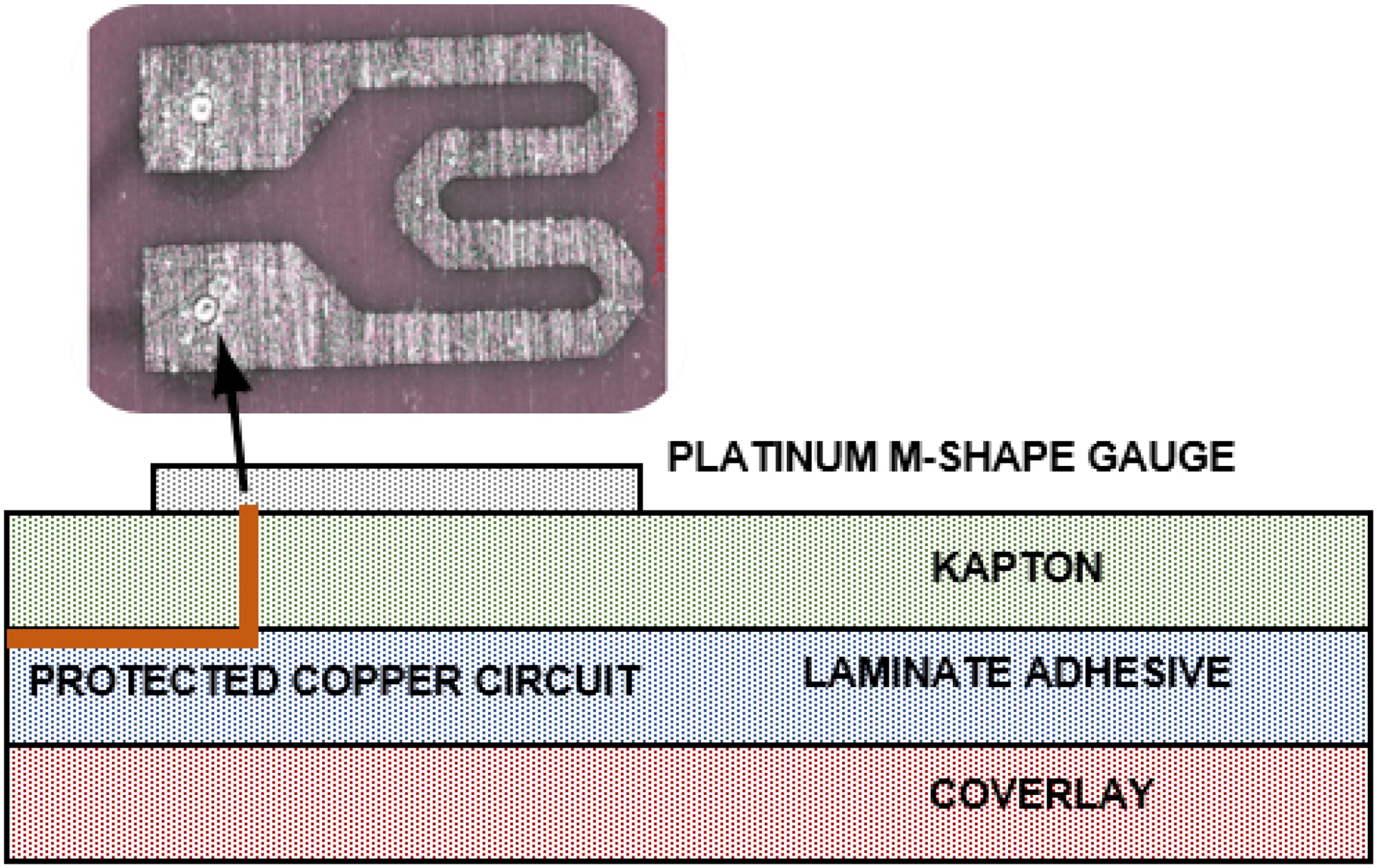
Thin film technology has advanced significantly since the work of Doorly. Collins et al. (2015), Shaikh (2020) introduced new manufacturing techniques using commercial flexible element PCBs, Figure 2. The upgraded manufacturing methods introduce interstitial or coverlay laminates in the thin film construction, which enables complex circuitry to be embedded in the PCB. Combined with high accuracy production tolerances, these new designs offer a higher density of thin films on the active surface. Along with the internal adhesive, main fixing adhesive and test geometry substrate, modern thin film analysis should always be considered a multilayer system. The following section outlines the general equation for the surface temperature of an N-layer laminate with applied unit surface heat flux.

Figure 2.

Schematic of a modern day thin film laminate construction used at the OTI.

Boundary condition method

Following the process used by Oldfield in the two layer case, the laminate basis functions are derived starting with a Laplace transform of the Fourier conduction equation. Beginning at the lower most laminate layer, N, interface boundary conditions are propagated upwards through the laminate to the known upper surface boundary condition, Figure 3. The method assumes the back substrate can be considered semi-infinite, the heat flow is one dimensional and the system is initially uniform zero temperature.

Figure 3.

Section through a multilayer, semi-infinite laminate showing boundary and continuity conditions.

(1)

∂2ϕ∂x2−sαϕ(x,s)=0

(2)

ϕN(x,s)=AN(s)e−xs/α

(3)

ψN(x,s)=ks/αAN(s)e−xs/α

The following interface boundary conditions are defined, with variable substitutions: An=An(s),Bn=Bn(s),λn=s/αn

• Temperature continuity

(4)

AN−1e−xN−1λN−1+BN−1exN−1λN−1=ANe−xN−1λN

• Heat flux continuity

(5)

kN−1λN−1AN−1e−xN−1λN−1−kN−1λN−1BN−1exN−1λN−1=kNλNANe−xN−1λN

Introducing the variables σm,n and γm,n

(6)

σm,n=knλnkmλm,γm,n=1−σm,n1+σm,n

Multiplying 4 by σ and subtracting 5, the following relation is found, allowing BN−1 to be found in terms of AN−1

(7)

(1−σN−1,N)AN−1e−xN−1λN−1=(1+σN−1,N)BN−1exN−1λN−1

(8)

BN−1=AN−1e−2xN−1λN−1γN−1,N

Moving up one layer in the laminate stack, the temperature and heat flux conservation is given by

(9)

TemperaturecontinuityAN−2e−xN−2λN−2+BN−2exN−2λN−2=AN−1e−xN−2λN−1+BN−1exN−2λN−1

(10)

HeatfluxcontinuitykN−2λN−2AN−2e−xN−2λN−2−kN−2λN−2BN−2exN−2λN−2=kN−1λN−1AN−1e−xN−2λN−1−kN−1λN−1BN−1exN−2λN−1

Substituting variables σ, λ and BN−1, then multiplying 9 by σ, the two continuity equations above become 11 and 12. Noting that xn is the spatial position of the back surface of layer n, (xN−1−xN−2) defines the thickness of layer N−1.

(11)

σN−2,N−1AN−2e−xN−2λN−2+σN−2,N−1BN−2exN−2λN−2=σN−2,N−1AN−1e−xN−2λN−1[1+γN−1,Ne−2(xN−1−xN−2)λN−1]

(12)

AN−2e−xN−2λN−2−BN−2exN−2λN−2=σN−2,N−1AN−1e−xN−2λN−1[1−γN−1,Ne−2(xN−1−xN−2)λN−1]

Multiplying the temperature Equation 11 by the RHS [] term in the flux equation and multiplying the flux Equation 12 by the RHS [] term in the temperature equation. The RHS of the above two equations become equal and 11 is equated to 12. This can be rearranged to find BN−2 in terms of AN−2

(13)

BN−2=AN−2e−2xN−2λN−2(1−σN−2,N−1)+(1+σN−2,N−1)γN−1,Ne2xN−2λN−2(1+σN−2,N−1)+(1−σN−2,N−1)γN−1,Ne2xN−2λN−2

This equation has the same form as 8 and can be written

(14)

BN−2=AN−2e−2xN−2λN−2ηN−2,N−1

whereηN−2,N−1=γN−2,N−1+γN−2,N−1e−2(xN−1−xN−2)λN−11+γN−1,NγN−1,Ne−2(xN−1−xN−2)λN−1

The process from 9 to 14 can be repeated for all additional layers in the laminate. For each layer above N−2, the relation ηm,m+1 is based on the value of η in the below layer and γ of the current layer. Once this process has propagated to the top surface of the material stack. The surface temperature and flux boundary conditions can be applied.

(15)

ϕ(0,s)=A1+B1

(16)

ψ(0,s)=k1λ1A1−k1λ1B1

Substituting B1 from 14 into the above surface conditions gives

(17)

A1=ψ(0,s)k1λ1[11−η1,2e−2x1λ1],B1=ψ(0,s)k1λ1[η1,2e−2x1λ11−η1,2e−2x1λ1]

ϕ(0,s) can then be rearranged and expanded as a power series, giving the final Laplace domain surface temperature solution.

(18)

Powerseries,11−z=∑i=0∞⁡zi;|z|<1

(19)

ϕ(0,s)=ψ(0,s)k1λ1[1+2η1,2e−2x1λ11−η1,2e−2x1λ1]

(20)

ϕ(0,s)=ψ0k1λ1[1+2∑i=1∞⁡η1,2ie−2x1λ1i]

Expanding the numerator and denominator as separate binomial series, η can be expressed as a product of summations.

(21)

ηm,m+1i=[∑j=0i(ij)γm,m+1i−jηm+1,m+2je−2j(xm+1−xm)λm+1]×[∑k=0∞(i+k−1k)(−1)kγm,m+1kηm+1,m+2ke−2k(xm+1−xm)λm+1]

The above product can be combined to give an infinite sum of a finite series. For progressive terms in the infinite summation, the exponential term tends to zero. The infinite series can therefore be accurately approximated by a truncated finite series of length k. Truncation is recommended when the value of η falls below a defined negligible value, this is material dependent and should be defined on a case by case basis. A typical value for negligible consideration is a summation term <10−6, typically corresponding to a truncation index of k=5.

(22)

ηm,m+1i=∑k=0∞⁡[∑j=0i⁡(ij)(i+k−1k)(−1)kγm,m+1i−j+kηm+1,m+2j+ke−2(k+j)(xm+1−xm)λm+1]

The formulation of ηm,m+1 depends on the the next layer value of ηm+1,m+2. This variable must therefore be progressively substituted until the solution propagates down through the laminate. Each time this variable is replaced, a dual summation of the ηm+1,m+2 term in the next layer is required. This substitution is continued until m>N−2 where the value of η depends only on γ and is fully defined by the material properties. This approach leads to a final solution with 1+2(N−2) nested summations containing the material properties and thickness of each laminate layer.

The above solution is rather involved and becomes increasingly unwieldy as the laminate grows. Due to the effect of layer count on the number of nested summations, implementing this approach is non-trivial, even on simple laminates. The simulation of an 8-layer case, required for more complex thin film constructions, can take several hours to process due to the nested loop formulation. Practical use is therefore not recommended for cases other than simple laminates with low layer count. In the single and two layer cases, the nested summations drop out, leaving a simplified form identical to those presented by Oldfield.

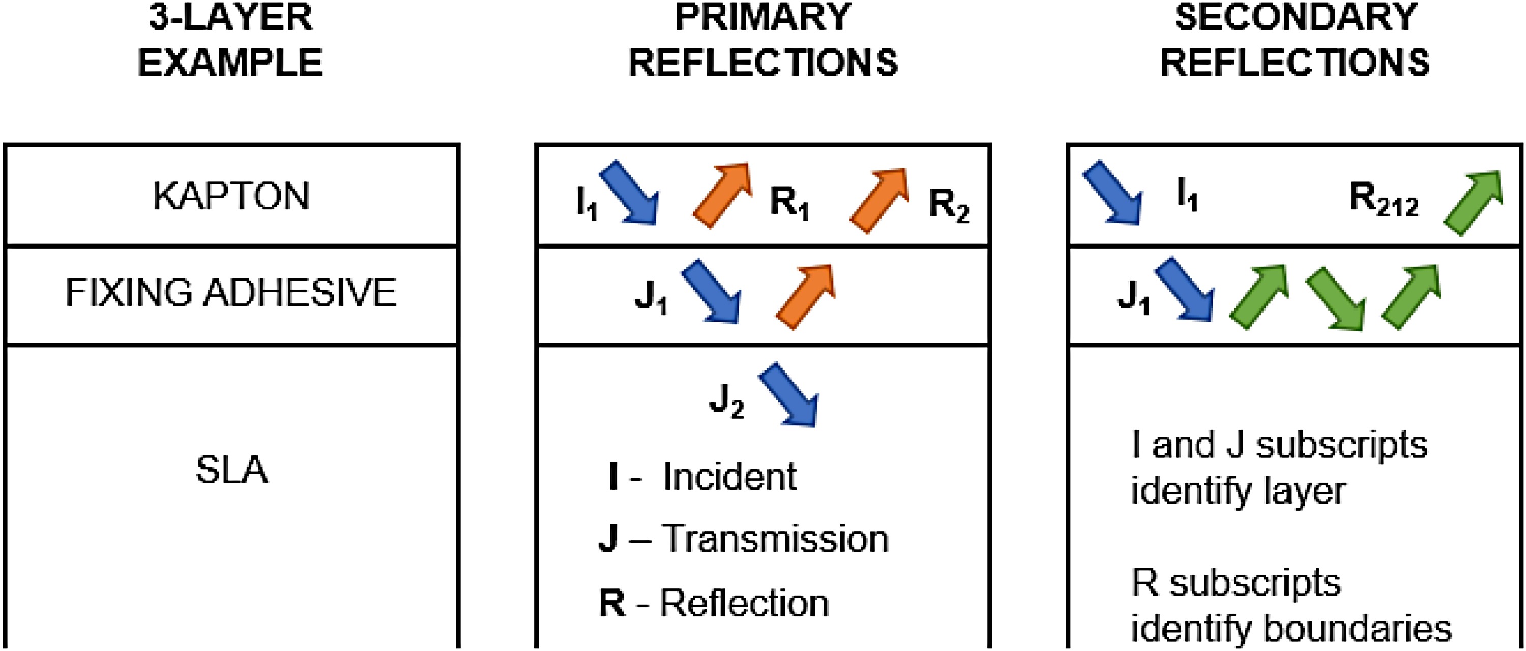
Transmission-reflection method

When handling more complex constructions, an alternative more user friendly method is preferred. In practice, many of the summation terms in the above solution can be considered negligible and only the significant terms need be considered. Similar to the transmission and reflection of electromagnetic waves at a material interface (Lekner, 2016), heat penetration through a laminate can be solved in the same way. The incident heat at the material interface is partially transmitted to the next material and partially reflected to the original material. This is seen as a change in the thermal gradient, affecting the heat flux through each layer. These split thermal profiles continue to propagate through the laminate, splitting again at each interface. Beyond the secondary reflections, the magnitudes can be considered negligible and a simplified approximate solution can be found. Solved at the surface, x=0, the temperature profile is simply the sum of the incident function and any reflected terms seen at this location. The transmission-reflection process for a three layer laminate is outlined in Figure 4.

Figure 4.

Transmission-Reflection method applied to a three layer laminate, showing the primary and secondary reflections.

Solving the direct unit step analytic solution adds unnecessary complication. Instead, any solution pair for temperature and heat flux may be found, then simply converted to the unit step solution afterwards if required. This is easily done using the impulse response; the filter H(s) from the known heat flux solution to a unit step can be found, then applied to the corresponding known temperature. This method allows the easiest analytic solution pair to be used and further simplifies the approach. Similar to the boundary condition solution, this is best implemented in the Laplace domain then inverted later to find the time domain form.

(23)

ϕunitstep(s)=H(s).ϕknown(s);whereH(s)=ψunitstep(s)ψknown(s)

Any definition for the incident function, I1, may be selected. The parabolic surface temperature for an isotropic material is recommended as the simplest form, and yields the easiest final temperature and heat flux solutions.

(24)

I1(x,s)=1s3/2e−xs/α1

At the first interface, x=x1, the incident function is split according the transmission and reflection coefficients.

(25)

CTij=2nini+nj;CRij=ni−njni+nj;whereni=ki/αi

The transmitted part, J1, progresses to the next material and is formed of the following components

• the transmission coefficient, CT12

• the initial surface function, 1/s3/2

• the diffusion in the current layer, exp(−[x−x1]s/α2)

• the diffusion from the previous layer, exp(−x1s/α1)

(26)

J1(x,s)=CT121s3/2e−(x−x1)s/α2e−x1s/α1

The reflected part, R1, travels backwards in the first material and is formed of the following components

• the reflection coefficient, CR12

• the initial surface function, 1/s3/2,

• the diffusion in this layer, exp(−[2x1−x]s/α1)

(27)

R1(x,s)=CR121s3/2e−(2x1−x)s/α1

Note that at the first boundary interface, x=x1, the following equality applies

(28)

I1(x1,s)+R1(x1,s)=J1(x1,s)

The transmitted part then progresses to the next material. Applying the reflection and transmission coefficients at each subsequent boundary, the remaining reflection terms from Figure 4 can easily be found

(29)

R2(x,s)=CT12CR23CT211s3/2e−(2x1−x)s/α1e−2(x2−x1)s/α2

(30)

R212(x,s)=CT12CR23CR21CR23CT211s3/2e−(2x1−x)s/α1e−4(x2−x1)s/α2

The final surface temperature solution, ϕ(0,s), is given by the sum of all terms present at this location, x=0.

(31)

ϕ(0,s)=I1(0,s)+R1(0,s)+R2(0,s)+R212(0,s)

The heat flux, defined by −k1dT/dx, can be found by spatial differentiation

(32)

ψ(0,s)=k1α1s[I1(0,s)−R1(0,s)−R2(0,s)−R212(0,s)]

The following Laplace transform inversions can be used to find the time domain solution for heat flux and temperature (Abramowitz and Stegun, 1972).

(33)

1se−as⇔erfc(a2t)1s3/2e−as⇔2tπexp(−a22t)−aerfc(a2t)

The time domain form for both temperature and heat flux are therefore a sum of factored exponential and complimentary error functions. The factors are given by the product of transmission and reflection coefficients, the erfc and exp terms are given by the sum of the dxi/αi ratio in each layer passed through. The example three layer solution for surface heat flux and surface temperature are given below.

(34)

q(0,t)=k1α1[erfc(0)−CR12erfc(a2t)−CT12CR23CT21erfc(b2t)−CT12CR23CR21CR23CT21erfc(c2t)]

(35)

T(0,t)=2tπ+CR12[2tπexp(−a22t)−aerfc(a2t)]+CT12CR23CT21[2tπexp(−b22t)−berfc(b2t)]+CT12CR23CR21CR23CT21[2tπexp(−c22t)−cerfc(c2t)]wherea=2x1α1,b=2x1α1+2(x2−x1)α2,c=2x1α1+4(x2−x1)α2

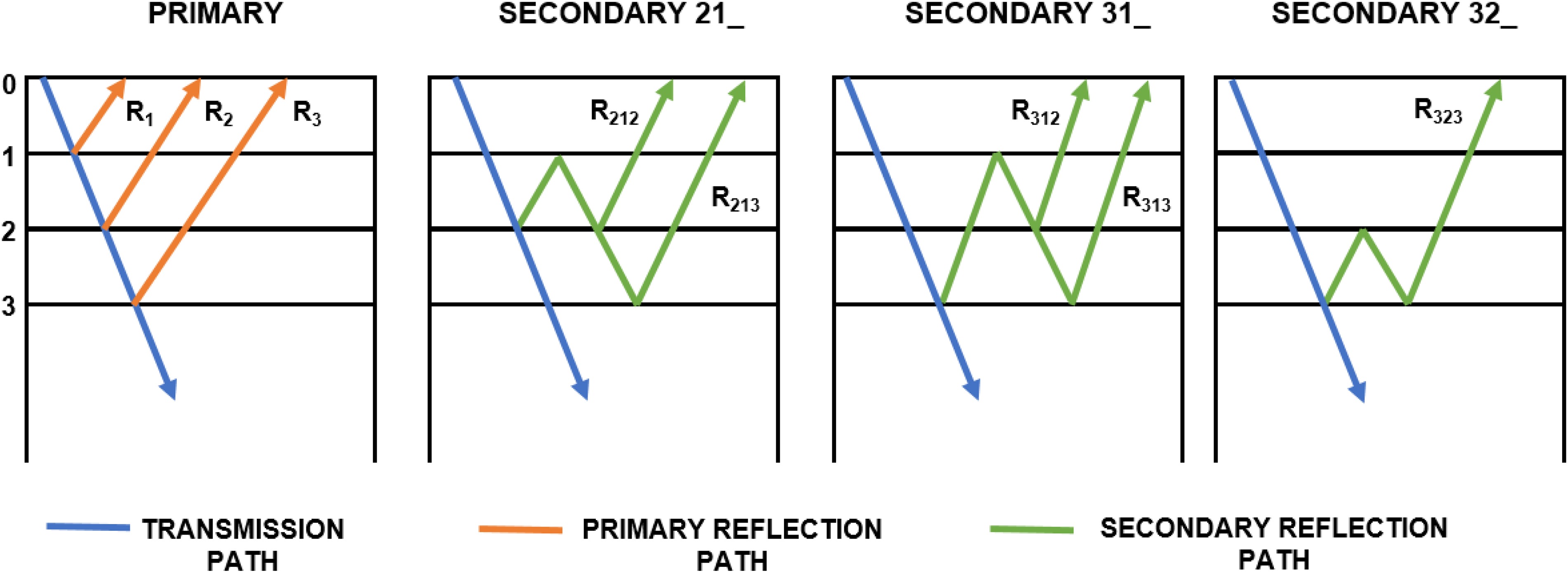
For higher layer counts, internal reflections occur at all layers in both the upward and downward direction. To accumulate all secondary reflections, three nested for loops are required in the analysis code.

• Loop one, define all first upward reflections, one at each material interface below the surface, i = 1: N − 1.

• Loop two, define all first downward reflections, one at each layer above the current ith layer, j=1:i−1.

• Loop three, define all second upward reflections, one at each layer below the current jth layer, k=j+1:N−1.

The product of each transmission and reflection coefficient, along with the factors for the erfc and exp terms, can be routinely collected within each loop. This method can thus be programmed with a static code structure and is substantially easier to implement than the previously discussed boundary condition solution, with 1+2(N−2) nested summations. The transmission-reflection method is universal, allowing a laminate of any layer count to be automatically handled by the simple loop coefficients. The straightforward three loop implementation yields sufficient accuracy in this case however, if further accuracy is desired, users may add additional loop pairs to capture tertiary or higher order reflection terms.

Higher layer count laminates are handled in exactly the same way. A four layer laminate is shown in Figure 5, highlighting the captured reflection terms by the simple three loop model. Similar to the example three layer case above, the surface functions are given by the sum of terms present at x=0.

Figure 5.

Reflection paths in a four layer laminate that are automatically handled by the standard three loop method.

(36)

ϕ(0,s)=I1(0,s)+R1(0,s)+R2(0,s)+R212(0,s)+R213(0,s)+R312(0,s)+R313(0,s)+R323(0,s)

(37)

ψ(0,s)=k1α1s[I1(0,s)−R1(0,s)−R2(0,s)−R212(0,s)−R213(0,s)−R312(0,s)−R313(0,s)−R323(0,s)]

Analytic results and discussion

The analytic solutions using the transmission-reflection method have been evaluated for a single, two, three and five layer laminate, Figure 6, with applied unit step surface heat flux ψ(0,s)=1/s. The three and five layer cases examine the construction of a laboratory thin film test, where a polyamide kapton circuit is adhered to a 3D printed SLA test geometry. 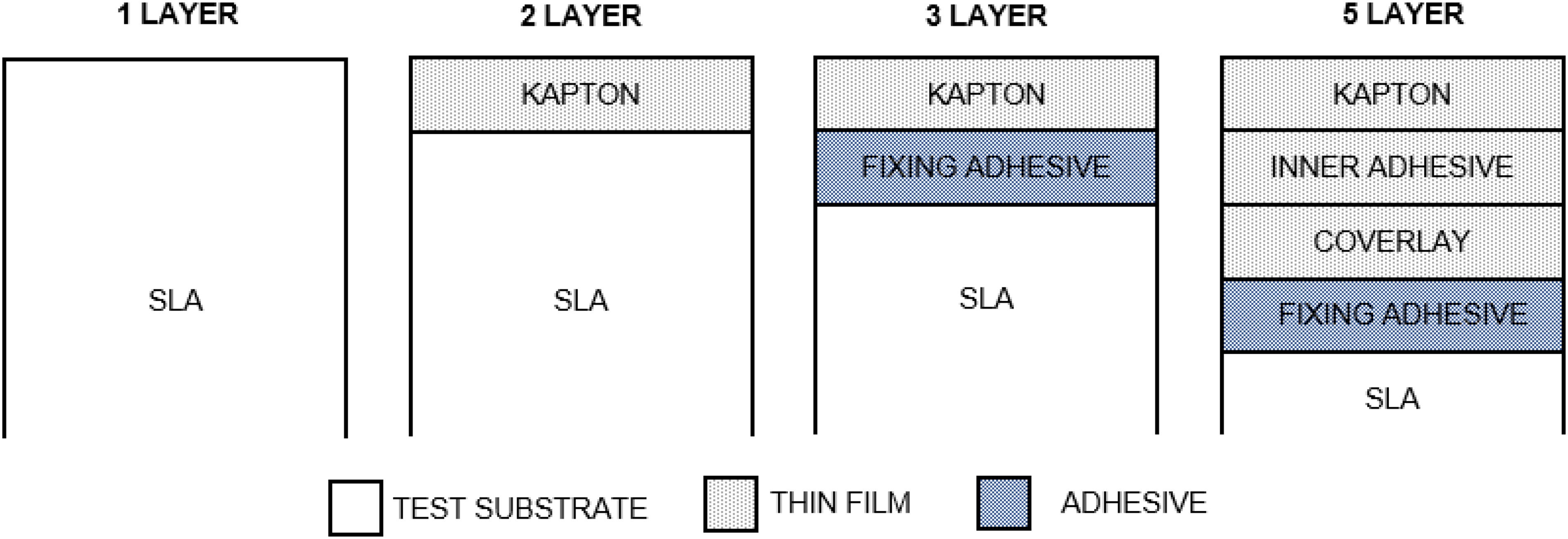The material properties considered in this analysis are shown in Table 1.

Figure 6.

The four analysis cases showing the material construction for the different layer models.

The kapton and adhesive layers are significantly thinner than the SLA geometry and, under traditional application of the impulse response method, would be ignored. Figure 7 shows the surface temperature function required to generate unit step heat flux under different combinations of these materials. Due to the lower thermal product of kapton and the fixing adhesive, a higher surface temperature is required to achieve unit step heat flux in these materials.

Figure 7.

Surface temperature required for unit step heat flux, with the derived impulse response filter for the four different laminate layer cases and the calculated heat flux when applying each response function to T5.

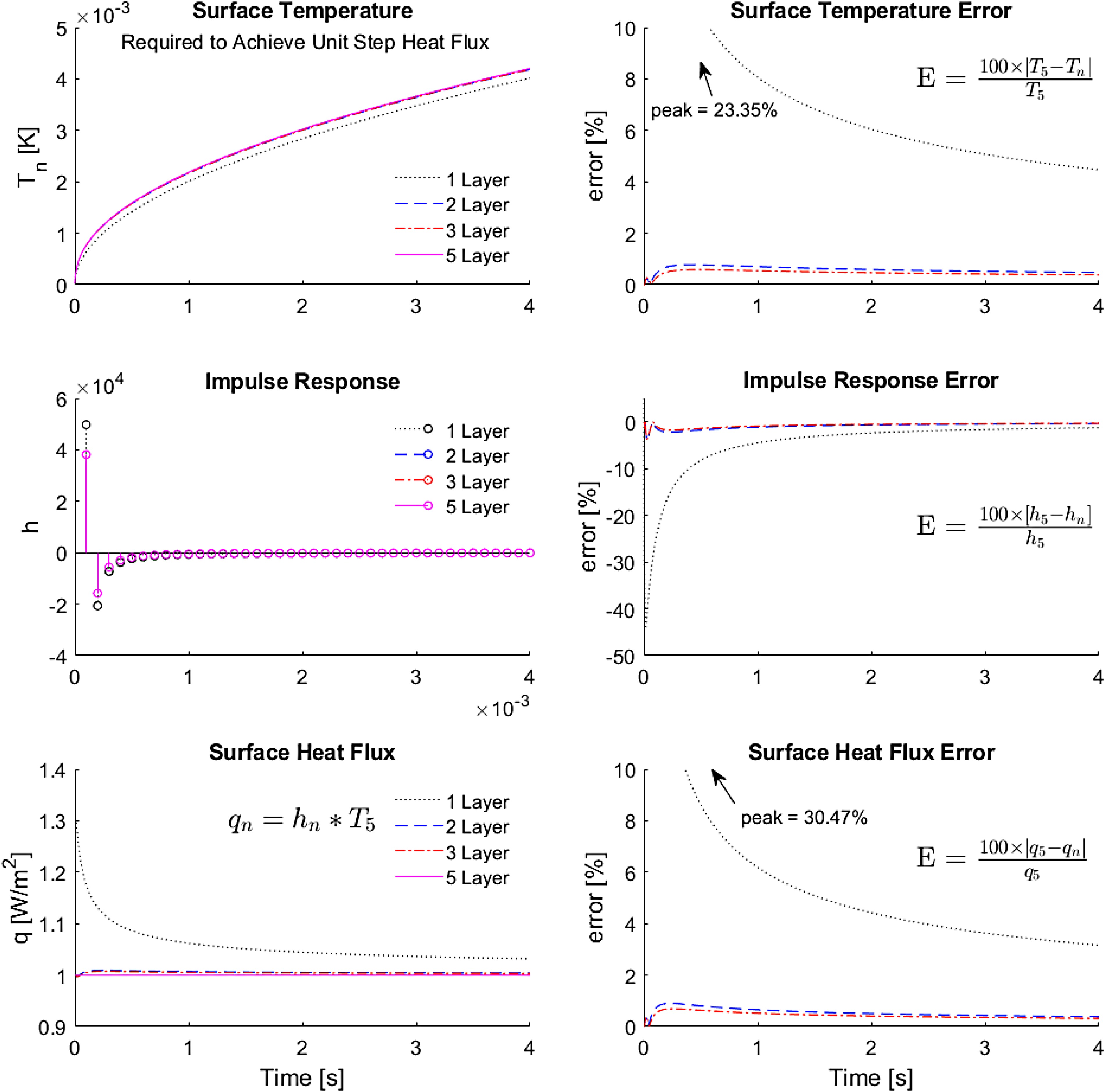
The impulse response filter is defined by a known basis function pair for temperature and heat flux. If the upper layers are ignored, an incorrect surface temperature function is used to solve the filter. The error is thus directly built into the analysis filter and effects the accuracy of the post-processing only.

When applying the impulse response method, the physically measured surface temperature is post-processed with the response filter to find the heat flux. The impact of the embedded error is thus seen in the calculated flux value. Figure 7 shows the effect when the response filter is calculated using each of the different layer models. In all cases the calculated filter is applied to the five layer surface temperature, T5layer. This solution best replicates the true geometry and thus best replicates the actual surface temperature that would be measured in a unit step heat flux test.

As seen in Figure 7, when using the simplified filters (h1,h2,h3) the heat flux is overestimated, particularly during the early part of the analysis. This error reduces with time as the thermal profile penetrates past the additional layers and the back substrate material dominates. The value and duration of the large error region depends on the material properties and thermal penetration time of the additional laminate layers and must be evaluated on a case by case basis.

In this typical thin film construction, the impact of a single layer assumption is significant for the full duration of the test. Using the simplified impulse response leads to large errors in the calculated heat flux. Peak error in the heat flux calculation is 30.47%, reducing to 3.62%, with a time averaged value of 6.71%. Despite the thin nature of the additional layers, and approximately similar thermal properties, the error caused by simplifying the post-processing method is significant. When using the two or three layer impulse response, the error is notably better than the single layer case. In all cases where the test article has a laminate construction, with differing material properties, the impulse response should be derived from the multilayer system response to prevent large errors being inherited in the filter.

The discussed example focuses on the calculation of surface heat flux from surface temperature. It should be noted that the impulse response can be taken between any two analytic temperature or heat flux functions i.e. one could equally map the temperature and heat flux between different layers in the laminate and infer positional offset in the response function. The transmission-reflection method is equally applicable by simply collecting the active terms at each spatial position. Provided the full system remains linear time invariant, the laminate methodology is not restricted to surface calculations and fully supports subsurface embedded temperature measurements.

Manufacturing assessment

The analysis above requires detail knowledge of the thermal properties and thickness of each layer. Accurate measurement of the thermal conductivity, especially in thin polyamide materials, is well known to have notable error bounds. Li (1990) estimates the statistical uncertainty of TC-1000 thermal comparator measurement techniques to be in the region ±15% on films above 25.4μm. Noting that the square root of the thermal conductivity is always referenced in the formulae, the full impact of this uncertainty is not seen in the heat flux calculation.

The formulae include the thermal product of the material k/α=ρkcp. Measurement of the additional properties is significantly more accurate; density measureme ±0.05% (American Society for Testing and Materials, 2012) and specific heat capacity measurements using DSC methods are within nts to ASTM D-1505 are within ±3% Bernardes et al. (2020). Taking the maximum and minimum values of each property in the thermal product, the uncertainty in this value can be calculated as ±9.4%. Given the Laplace domain transfer function from temperature to flux is factored directly by the thermal product, this corresponds to the single layer material uncertainty in the impulse response calculation.

Modern-day thin films are manufactured as part of a flex circuitry panel, with several sensors cut from the same manufacturing run. The construction tolerances in Table 1 are considered. These are consistent across the panel and in cases where higher accuracy is required, a sacrificial sensor or dedicated coupon may be sectioned to measure the executed laminate thickness. The substrate layer is considered semi-infinite, so thickness tolerances of this layer may be ignored.

Table 2 shows the calculated bounds of the uncertainty caused by material and construction tolerances in the five layer laminate case. In each construction, the same surface temperature was applied to the laminate, corresponding to the profile for unit step heat flux in the nominal tolerance case T5, shown in Figure 7. The calculated heat flux, for each combination of material and thickness tolerance, was compared to the true unit step value. Table 2 shows the peak difference and RMSE in the calculated heat flux, when using the impulse response method. As seen in the data, the impact of thickness tolerance is negligible, peak 0.34% and RMSE 0.16%, and could reliably be ignored in thin film testing.

The material property effects dominate, with a peak discrepancy of 10.35% and RMSE 9.82%. This is slightly higher than the thermal product uncertainty, 9.4%, due to the additional effects in the transmission and reflection coefficients at the material interfaces. However, the thermal product value gives a good indication of the behaviour in the full laminate.

The uncertainty values are comparable in magnitude to the time averaged error of the single layer assumption. However, even the combined worst case manufacturing uncertainty, 10.35%, is significantly less than the peak error, 30.47%, introduced by using the incorrect layer construction for the impulse response calculation. Where possible the material properties should be closely controlled however, priority should be given to removing the known error source and using the correct multilayer response filter.

1D multilayer numerical methodology

The derived analytic solutions are rather involved, particularly for the boundary condition method. In addition, these solutions have limitations in the handling of time varying material properties and back surface boundary conditions. Direct numerical methods allow for both of these limitations to be bridged and can offer comparable accuracy at the cost of computational effort. Battisti and Bertolazzi (n.d.) used a 1D finite element scheme with temperature dependent material properties. This method was validated on a single layer isotropic material and showed comparable accuracy.

Recktenwald presented several numerical methods, with differing stability dependent on the spatial and temporal discretisation (Recktenwald, 2011). The Crank-Nicolson algorithm was demonstrated with unconditional stability. The method uses a weighted average of the forward and backward time difference on the discrete centre space calculation. It is implicit with second order truncation errors in both time O(Δt2) and space O(Δx2). Although computationally more expensive per time step, its unconditional stability can allow for larger time steps without divergence.

When separated into the temporal components, the Crank-Nicolson method results in a tri-diagonal matrix equation on either side of the equality. This is commonly solved using a row reduction matrix inversion on the left hand side. The matrix is easily inverted using the Thomas algorithm or equivalent, which is computationally efficient with O(nx2) and available via Mathworks Exchange Holmes (2021).

Extending this method to a multilayer system, one must ensure that the heat flux is conserved at the interface boundaries. Hickson et al. (2011) presented a Taylor series expansion method for ensuring flux continuity at a laminate interface. Coefficients of nodes at locations [−2Δx,−Δx,0,Δx,2Δx] are used, where Δx is the distance from the interface boundary. Adapted to the Crank-Nicolson scheme, this can be concisely written as a penta-diagonal matrix. To maximise sparsity and reduce the computational effort, the bulk of the solver follows the traditional Crank-Nicolson method, with only the interface nodes modified for cross boundary heat flux continuity. The solver is applied to a 1D discretised domain with time stamps, m, and spatial positions, i.

Below is the modified multilayer penta-diagonal scheme, for a discretised domain [i,n], with a laminate boundary at i = 3:

Due to the sparse nature of both the left and right side solver matrices, this equation can be stored in vector form extracting only the populated diagonal vectors a,b,c,d,eandf along with the temperature vectors Tm−1andTm. The penta-diagonal matrix can be solved efficiently using a row reduction algorithm conceptually similar to the Thomas algorithm, Askar and Karawia (2015), Benkert and Fischer (2007). The method can be accelerated by pre-computing the algorithm factors σ,ϕ,ω,ρandψ and reusing these during each iteration. This acceleration technique is only valid if the material properties, spatial step and temporal step remain constant throughout the simulation. In such cases, the method can additionally be parallelised by stacking temperature vectors horizontally and applying the row-wise algorithm to all temperatures simultaneously. This is recommended when analysing infra-red thermography, allowing concurrent post-processing of multiple pixels. The penta-diagonal inversion algorithm applies successive row operations to reduce the LHS matrix to a lower diagonal form. The RHS is then solved by standard matrix multiplication to give the vector ω, followed by forward substitution of the diagonal LHS.

Numerical results and discussion

The penta-diagonal scheme has been validated against the same analytic solutions used in the impulse response method above. The spatial gradient from the temperature vector was used to extract the numerical heat flux at the surface. Figure 8 shows the performance of the numerical scheme, along with a comparison to the impulse response results. Following the same process as the data in Figure 7, the surface temperature for the five layer laminate, T5, was applied in each case. A numerical model was built for each of the different nominal laminates, using the same layer configurations and material properties as shown in Figure 6. The temperature was specified as an upper boundary condition in the numerical simulation. The extracted surface heat flux is then directly comparable to the calculation in Figure 7.

Figure 8.

Multilayer laminate heat flux comparison of the numerical penta-diagonal scheme and the impulse response solutions.

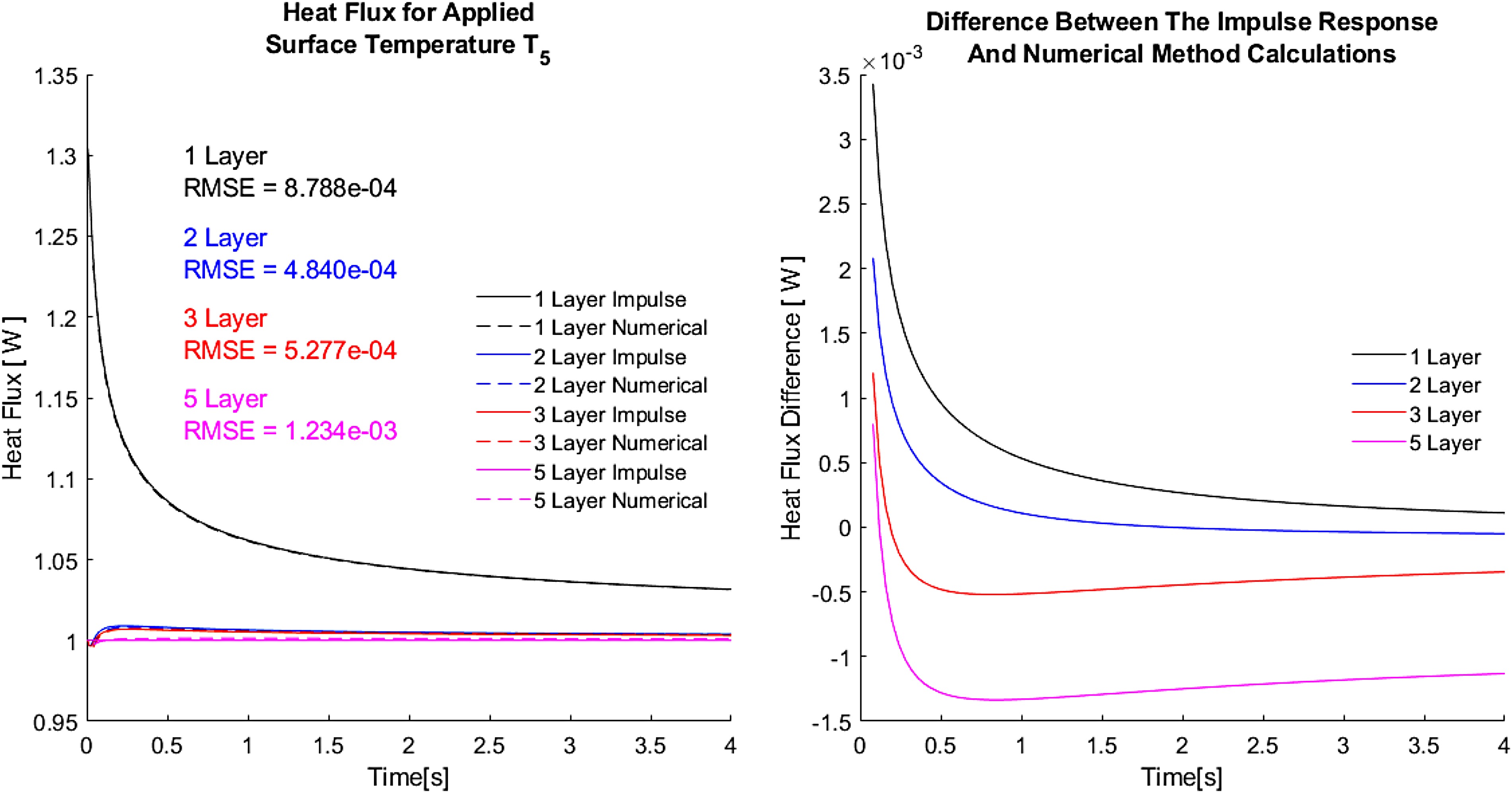
The calculated flux in the numerical model compares well to the reference impulse response. RMSE O(10−3) across all test cases confirms the suitability of the penta-digonal scheme for multilayer applications. The small difference is seen between the numerical result and impulse response due to the method of flux calculation in the numerical method. The spatial gradient is used in the calculation, which is dependent on the spatial interval of the numerical scheme. A trade off is required between accuracy and computation cost of the solver. Shown in Figure 8, the numerical result suffers most in the early time steps because the thermal gradient must first be established. This error is not seen in the impulse response because the method is better able to handle the step discontinuity in heat flux at time zero.

The performance of the numerical calculation can be improved by using a non-zero temperature profile to initialise the numerical scheme. An initial depth temperature profile equivalent to unit step heat flux over the first time interval, given by Equation 33, was used to improve the early flux calculation. The penta-diagonal method has suitable accuracy over the required data post-processing window and offers a valid alternative to the impulse response.

Figure 8 confirms the penta-diagonal scheme can be used to supplement or replace the impulse response calculation. It has the advantage that time varying material properties can be simulated and, a signal of any length or sampling frequency can be used without recalculation of the response filters. Control over both the front and back surface boundary conditions additionally allows the semi-infinite limitation to be removed, if this additional measurement data is available. The ability to support parallel post-processing of multiple sensors is a useful feature of the numerical approach. However, the small time step and spatial step required to support high frequency data sampling adds notable computational cost. Table 3 compares the features and capabilities of the discussed methods, showing the respective disadvantages and benefits of each.

Table 3.

Features and capabilities of the different methods to analyse multilayer heat transfer data.

Features and Capability	Single Layer Impulse Response	Multilayer Impulse Response	Multilayer Numerical
Calculation ease and simplicity
High speed frequency domain calculation
Support for parallel processing of many sensors
Support for advanced multilayer thin film gauges
Support for future embedded sensor measurements
Handle non-uniform or time varying material properties
Handle time varying back surface boundary conditions
Not restricted by the semi-infinite test duration
Variable frequency or signal length without padding

Conclusions

Heat flux measurements in short duration aero-thermal tests are commonly performed using the impulse response method. To simply the post-processing of this calculation, many users choose to assume a single, uniform, isotropic material and define the impulse response using the Oldfield unit step method. In reality, modern sensor constructions with test substrate and adhesives form a laminate with significantly different behaviour.

Multilayer analytic solutions were presented and validated, allowing direct calculation of the laminate surface functions. These solutions were used to analyse the impact of a single layer assumption. This common simplification introduced a 30.47% peak error with time averaged error of 6.71% over a four second test, corresponding to the permissible semi-infinite duration of the substrate in this case. These errors can be removed by simply replacing the impulse response basis functions with the correct multilayer solution. Two analytic solution methods have been presented and the second transmission-reflection method is easily implemented to find the upgraded filter inputs.

The uncertainty in impulse response analysis, arising from the thin film manufacturing tolerances, was analysed. The material thickness tolerances were shown to have negligible effect on the calculated heat flux. Variation in the material properties caused discrepancies ranging up to 10.35%. Although significant, this is notably less than the error caused by incorrect filter specification.

To support the calculation of time varying material properties, a numerical Crank-Nicolson method was also demonstrated for multilayer materials. This improved numerical scheme was validated against the analytic solutions and performed well across the test cases. Removing the semi-infinite and time invariant limitations, inherent to the impulse response, the numerical method offers a valid alternative for analysing heat transfer data.

Given the speed and simplicity of the impulse response method, in cases where the limitations of time invariance hold, this method should be preferred. Whenever possible, the response filter derivation should use the multilayer functions that best represent the true construction of the test article.

Nomenclature