Introduction

Centrifugal compressors are widely used in industry. With the advance of industries, centrifugal compressors with great capacity and high performance are required. However this type of centrifugal compressors with large flow coefficient is difficult to design and optimize (Zhu et al., 2016) due to complicated internal flow in the impellers. The traditional aerodynamic design and optimization method of impeller generally follows one-dimensional design, two-dimensional meridian channel design, quasi-three-dimensional blade design and full three-dimensional CFD verification. It requires not only the repeated numerical simulations for flow field analysis, but also iterations of the impeller geometry for continuous modifications. Although the traditional aerodynamic design method can achieve reasonable results, it needs manual debugging repeatedly, and greatly relies on the design experience of the designer, which is time-consuming. Thus, the combination between traditional aerodynamic design method and machine learning that have emerged in recent years has currently become a new direction of research.

Machine learning is a general term for a class of algorithms. We can use algorithms to mine the hidden laws in the data that cannot be processed by the human brain. As a branch of artificial intelligence, the machine learning is committed to study how to use computing to improve the performance of the system (Zhou, 2016). Its origin can be traced back to the basic tools of machine learning such as the least squares method and Markov chain in the 17th century. Its development has evolved through the connectionism in the 1980s, statistical learning in the 1990s, and deep learning in the 21st century. To date, the machine learning has become a new subject that integrates the theoretical foundations of multiple disciplines such as mathematics, computers, biology, and neurology. The interdisciplinary research related to machine learning is emerging, and some research results have already been transformed into practical applications.

With the continuous improvement of computing power and data volume, the rapid development of surrogate models such as artificial neural network models (Hassoun, 1996), kriging models, convolutional neural networks and recurrent neural networks has provided us with better tools to describe the relationship of “number-number”. In the design of centrifugal impeller, the relationship between the design parameters and aerodynamic parameters is mostly non-linear, which is difficult to be described by specific formulas. A new design method for centrifugal impellers is to use the surrogate model to construct a non-linear relationship and dig out the internal relationship.

In the process of centrifugal impeller design optimization, most optimization problems are not single-objective optimization problems, but multi-objective and multi-constrained global optimization problems. Therefore, gradient-based optimization methods are inherently unsuitable. The heuristic optimization algorithms such as evolutionary algorithm, particle swarm algorithm, annealing algorithm, ant colony algorithm, etc., have become important tools for solving such problems. These methods have developed rapidly in the field of machine learning in recent years. They are more suitable for solving multi-objective optimization problems, and better approaching the non-convex or discontinuous optimal front ends (Tang et al., 2004). A multi-objective genetic algorithm is a global algorithm that specifically solves multi-objective global optimization problems. It searches for the optimal solution by simulating the natural evolution process. In order to solve the problem of which the optimized sub-objectives may be contradictory, the concept of Pareto solution set is proposed. The optimization problems in this paper are all multi-objective global optimization, so the multi-objective genetic algorithm is selected (Deb et al., 2002).

Ibaeaki et al. (2015) and Verstraete et al. (2010) optimized a centrifugal impeller and diffuser by combining the surrogate model and advanced algorithms, and achieved good results. Guo et al. (2016) predicted the flow field of a centrifugal impeller based on the convolutional neural network. At the expense of partial accuracy, the computing speed was increased by two orders of magnitude. Duccio et al. (2002) optimized an impeller by combining the response surface and genetic algorithm, which greatly improved the aerodynamic performance of the impeller, but took too long time in the process. Kim et al. (2009) optimized the meridian flow channel of a centrifugal impeller through the radial basis function to improve its efficiency and total pressure ratio. These studies show the advantages and potential of machine learning methods for the design optimization of impellers machinery.

In this paper, the traditional design method of centrifugal impeller is combined with machine learning to design and analyze impellers with flow coefficients of 0.18, 0.2 and 0.22, which provides a new way for design of centrifugal impellers.

Methodology

Design and optimization process

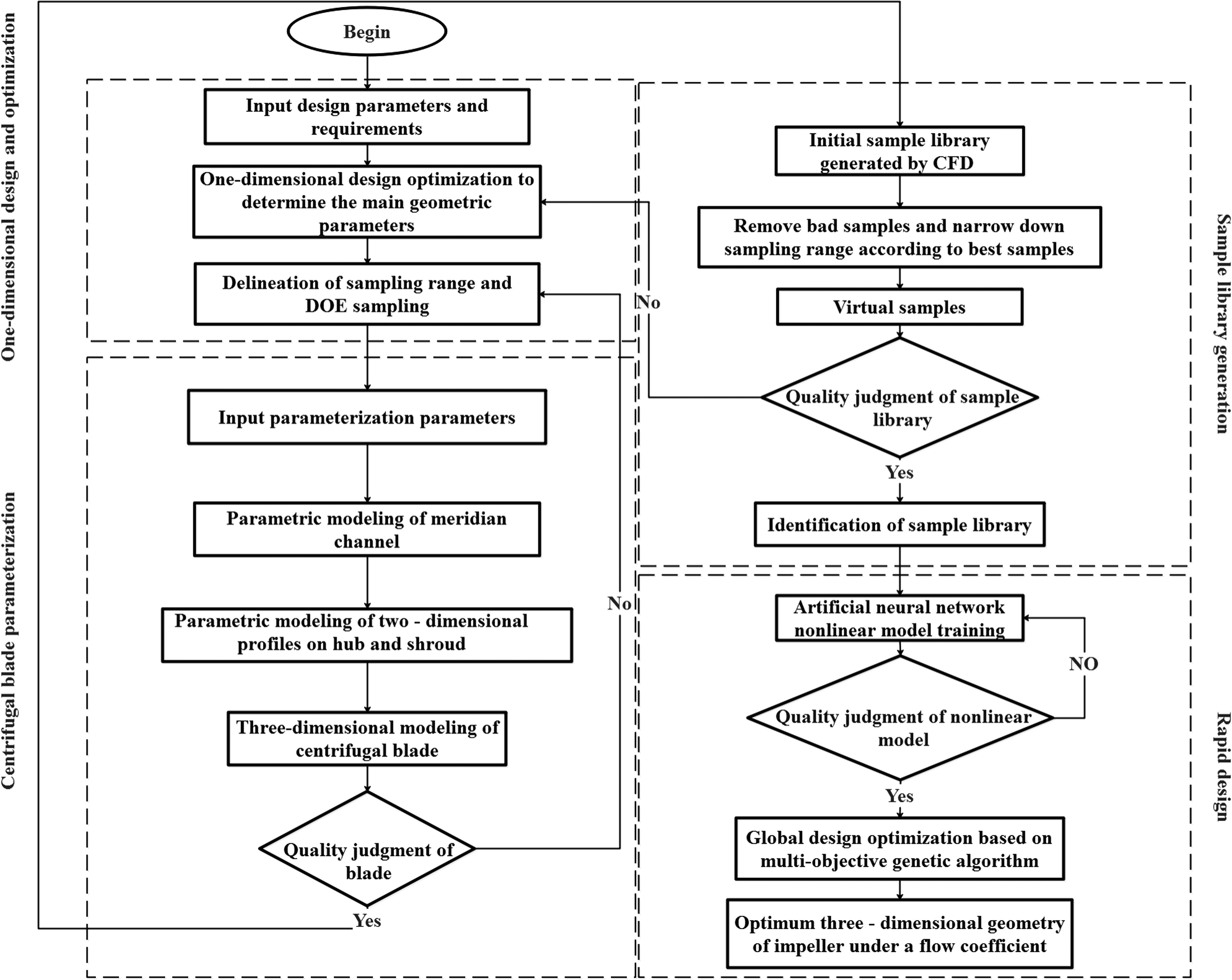
This section introduces the design and optimization process. Figure 1 shows the design and optimization flow chart, and gives the detailed introduction to the important parts.

1. First, input the design parameters and design requirements of the impeller, mainly including P₀, T₀, D₂, ɛ, n, q_m, Z, the fluid type, etc;

2. Based on the one-dimensional analysis program of the two-zone model and combined with the optimization algorithm, the specific values of the main one-dimensional geometric parameters (Gi) of the centrifugal impeller are obtained, including D_1s, D₂/D_1h, β_1s, β_1h, β₂, b₂, etc. The upper and lower bounds of each variable are determined according to the specific value in the initial sampling space;

3. Choose an appropriate design of experiment (DOE) to generate the initial sample parameters. In this study, the Latin superposition method was used for the initial sampling;

4. The meridian channel of the impeller blade, the β angle and the thickness of the blade on the shroud and hub are parameterized. Generate three-dimensional impellers according to the initial sampling parameters.

5. Qualified samples are calculated by CFD, the isentropic efficiency and total pressure ratio corresponding to each sample are obtained, and the sample library is initially generated. The samples are screened according to the sample with the best aerodynamic performance in the sample library. Re-determine the sampling range and repeat step 2 to screen and supplement the sample library;

6. The artificial neural network model is trained using the back propagation algorithm to construct a nonlinear model among the flow coefficient, geometric parameter control points, isentropic efficiency, and total pressure ratio.

7. The nonlinear model is used to replace the CFD calculation, and the multi-objective genetic algorithm is used for global optimization to achieve the rapid design of the centrifugal impeller;

8. Feedbacks are set up in the whole process to reduce the time of sample library construction and search, which is stated as follows:

   • Centrifugal blade parameterization part: check the requirements of the exit lean angle. The criterion is: exit lean angle <±20°;

   • Aerodynamic analysis part: check the isentropic efficiency, total pressure ratio and flow coefficient;

   • Non-linear model training part: check the value of the model correlation coefficient R. The closer R is to 1, the closer the sample value is to the 45 degree regression line. It shows that the higher the fitting accuracy, the better the regression effect. The criterion is R > 0.90.

Figure 1.

Design and optimization flow chart.

Parametric method of centrifugal impeller

A reasonable parameterization method of a centrifugal impeller should not be too complicated. While ensuring accuracy, it is better to use fewer parameter control points to reasonably describe the shape of blade. In order to achieve better coupling with the one-dimensional analysis program, an in-house parameterization program for centrifugal impellers has been developed in this study.

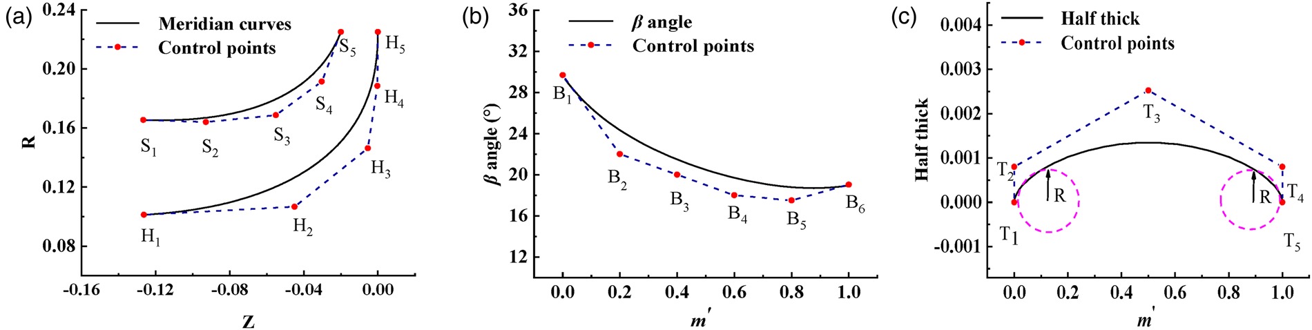
In the meridian coordinate system (R, Z), the meridian flow channel is given, and in the dimensionless meridian direction (m′, β), the β angle distribution is given. The β angle is converted into camber line through integration, and the thickness is superimposed on its normal direction to generate a two-dimensional blade shape. Finally, three-dimensional blades are generated by stacking the leading edges (Wang et al., 2019).

The flow condition of the main flow is determined by the meridian channel. As shown in Figure 2a, the meridian flow channel is composed of two meridian curves, both of which are constructed using 4th-order Bezier curves. The inlet and outlet geometry of the meridian curves is determined by the control points S₁, H₁, S₅ and H₅, and the remaining control points are used to adjust the shape of the meridian curves. Figure 2b shows the distribution of β angle at the hub, the β angle distribution of hub is constructed using 5th-order Bezier curves. The inlet and outlet β angle are respectively determined by the B₁ and B₆ control points, and the remaining control points are used to adjust the β angle distribution. Figure 2c shows the distribution of thickness at the hub, the thickness distribution of hub is constructed using 4th-order Bezier curves. T₂ and T₄ are used to control the shape of the leading and trailing edge, and their abscissas are the same as the control points of T₁ and T₅, respectively at the beginning and the end of the dimensionless meridian direction. T₃ is used to adjust the position and size of the maximum thickness. The parameterization method of β angle and thickness distribution of the shroud is the same as the hub. S_e (e = 1,…,5), H_f (f = 1,…,5), B_c (c = 1,…,12) and T_h (h = 1,…,10) respectively represent the control points and the corresponding coordinate values.

Figure 2.

Parameterization model of meridional channel (a), β at the hub (b), and thickness at the hub (c).

Sample library and training of nonlinear models

Design of experiment (DOE) plays an important role in the generation of the sample library, and a reasonable DOE method can make the sample distribution in the sample library more reasonable. Latin Hypercube is a stratified sampling DOE method. Compared with random sampling and full factorial design, it has a more effective space filling capacity on the basis of reducing sample requirements. For geometric parameters b₂, D_1s and the blade angle control points on the shroud and hub, Latin hypercube sampling was performed. The remaining parameters were selected based on the result of one-dimensional design optimization. Part of the control points of the β angle distribution and the meridian flow channel cannot be obtained through one-dimensional design and optimization. Therefore, in the initial sampling, a larger range is given, and the second sampling reduces the sampling range of the control points according to the optimal sample. After the sampling, three-dimensional samples are generated using the centrifugal impeller parameterization program.

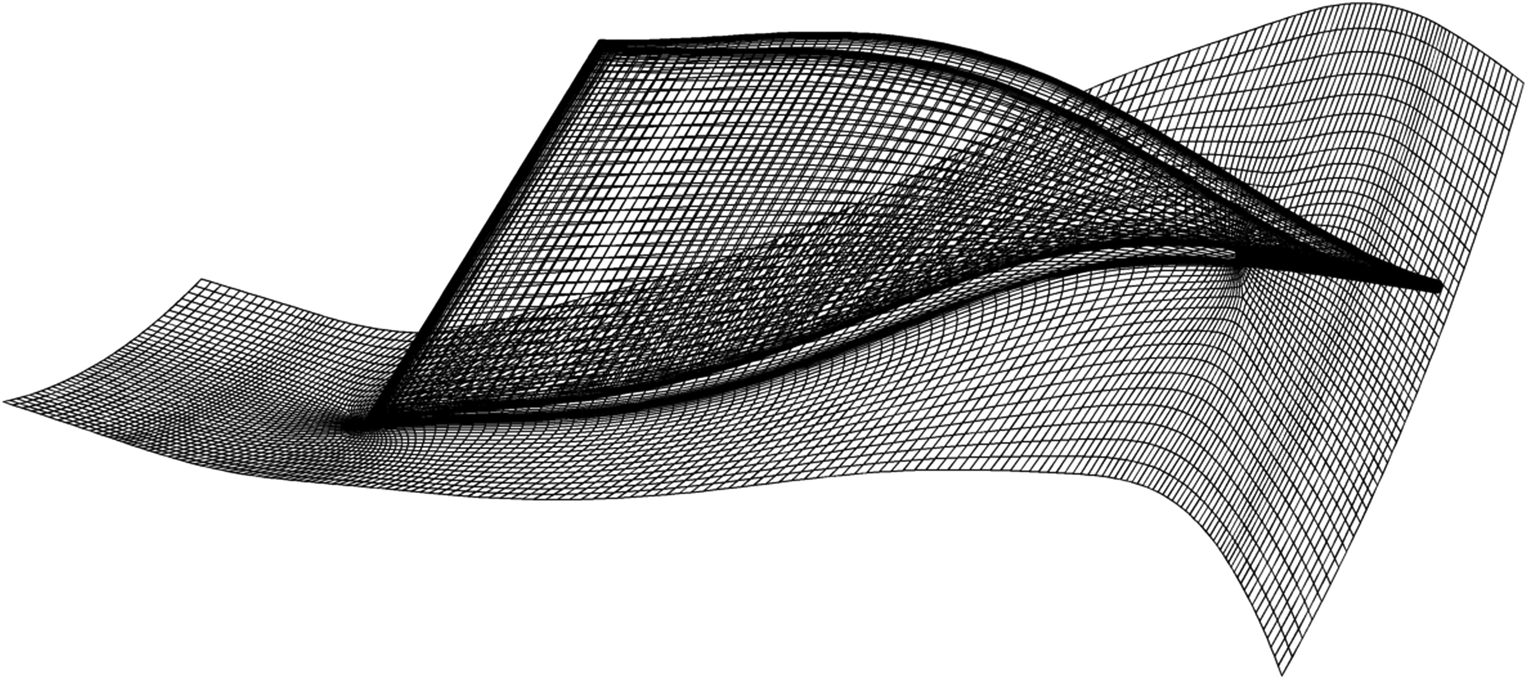
CFD calculation was performed on the three-dimensional samples of the centrifugal impeller. The grid was generated using the AutoBlade module of the NUMECA software. In order to trade off between calculation accuracy and computing cost, the grid number was set to 550,000. Figure 3 is shows the grid on the blade surface and the hub. The Fine module of the NUMECA software was used for numerical simulation, and the Spalart-Allmaras (SA) turbulence model was used.The chain of grid generation and flow calculation was automated using an in-house python script, thus to reduce manpower and time costs.

Figure 3.

Surface grid of the impeller.

According to the optimal sample in the initial calculation results, the sample space was reduced. Firstly, the samples were sorted based on the aerodynamic performance, and the non-convergent samples and the samples with poor aerodynamic performance were removed. Secondly, new ranges for the sample space were determined based on the optimal samples. Finally, new samples were filled. For the initial sampling, the number of samples in the sample library was 1,000. After removing samples and filling samples again, the total number of samples in the sample library became 463. Table 2 shows the second sampling range.

Table 2.

The second sampling range.

Design Variable	Lower Bound	Upper Bound	Design Variable	Lower Bound	Upper Bound	Design Variable	Lower Bound	Upper Bound
S1	0.039	0.043	B4	5	8	B9	50	58
S5	0.016	0.019	B5	12	21	B10	54	91
B1	45	57	B6	28	39	B11	27	45
B2	48	80	B7	42	51	B12	20	27
B3	10	17	B8	25	42	φ	0.18	0.22

The data was normalized, and the min-max standardization method was used to linearly transform the original data, so that the result could be mapped to 0–1, as shown in Equation 2.

(2)

Xnew=(X−Xmin)(Xmax−Xmin)

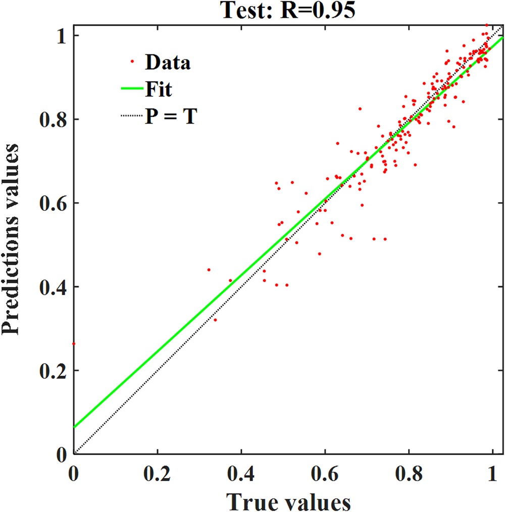
The ratio of the sample training set and the prediction set in the sample library is 0.15:0.85. After repeating tests, this research selected a 4-layer artificial neural network. BP algorithm was used to train artificial neural network. Figures 4 and 5 respectively show the model training curve and the test set 45-degree regression line (Lei, 2020). It can be seen that when the training epoch is about 70, the convergence is stable, and the mean square error of the training curve and the test curve are both less than 10⁻², which meets the convergence requirements. Most of the test samples are distributed around the diagonal of the 45-degree regression line, and only a few points are far away from the regression line. In addition, the regression coefficient R = 0.95, which is close to 1, indicating that the model has high fitting accuracy and strong generalization ability. Although there are still small deviations between the predicted aerodynamic performance of the model and the actual aerodynamic performance, it is difficult to find the actual optimal solution for complex problems with a large number of design variables, and a lot of computing costs are required. Considering the reduction of computing cost and design optimization cycle, these deviations can be considered acceptable (Zhang et al., 2018).

Figure 4.

Model training curve.

Figure 5.

Test set 45 degree regression line.

Results and discussion

The trained nonlinear model was combined with the multi-objective genetic algorithm for global optimization, and the impellers with flow coefficients of 0.18, 0.2 and 0.22 were designed respectively. The problem is mathematically formulated Equation 3. The basic parameters of the multi-objective genetic algorithm were set as follows: crossover probability 0.85, mutation probability 0.09, population size 150, and evolution generation 300 generations. After the convergence of algorithm, the best point was verified by CFD. The following is the analysis of results.

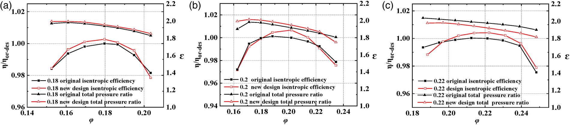
The impellers designed by machine learning CFD (new impellers) results were compared with the CFD results of original impellers. The original impellers were designed by a traditional method, and it had gone through a much longer design and optimization cycle than the new impellers. Figure 6 compares the variable condition performance curve of the new impellers and the original impellers with flow coefficients of 0.18, 0.2 and 0.22. It can be seen that at the design conditions, under the premise that the total pressure ratio meets the design requirements, the isentropic efficiency of the new impellers exceeds the original impellers and also the design requirements. After the main parameters of the impeller are obtained after rapid design, the optimization can be carried out for non-design conditions.

Figure 6.

Comparison of performance curves for different impellers. (a) φ = 0.18. (b) φ = 0.2. (c) φ = 0.22.

Figures 7–9 shows the relative Mach number contours and streamline at 10%, 50%, and 90% span of the impeller. It can be seen that the airflow is clean, and there is no obvious flow separation and shock wave phenomenon.

Figure 7.

Relative Mach number contours and streamlines of the impelller with a flow coefficient of 0.18. (a) 10% span. (b) 50% span. (c) 90% span.

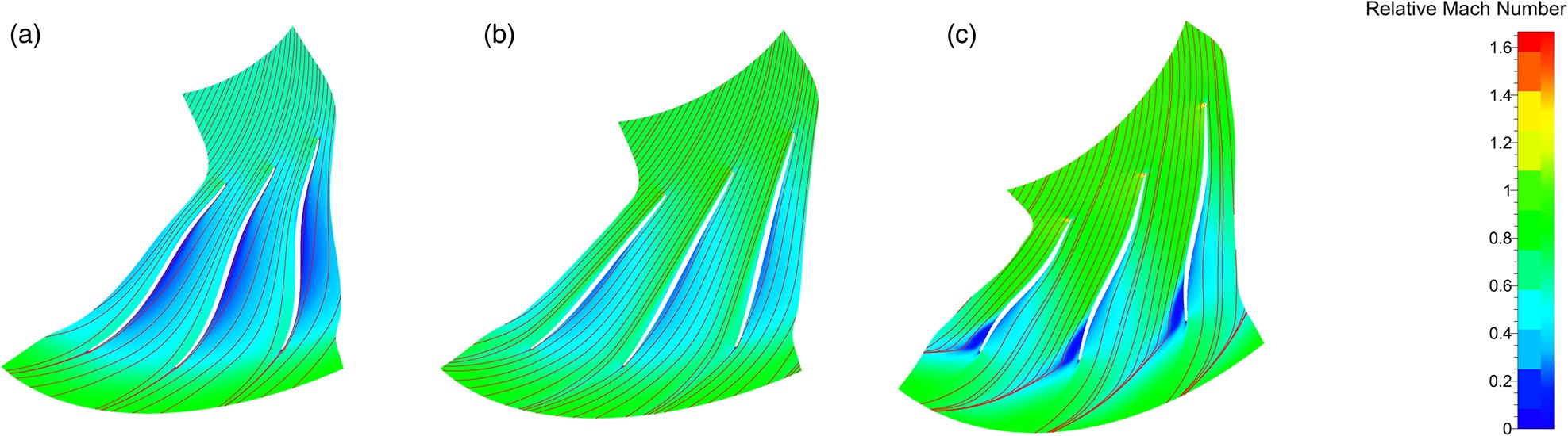
Figure 9.

Relative Mach number contours and streamlines of the impeller with a flow coefficient of 0.22 (a) 10% span (b) 50% span (c) 90% span.

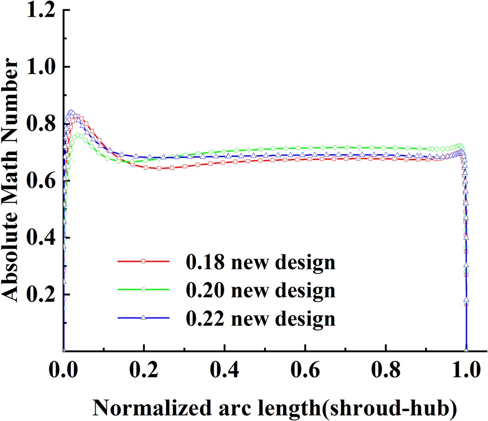
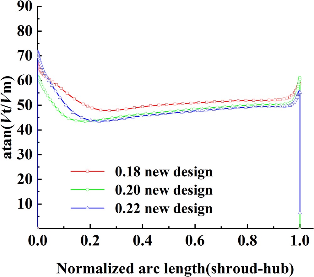
In order to study the uniformity of the airflow at the exit of the new impellers, Figures 10–12 respectively shows the absolute Mach number distribution, tangential velocity distribution and flow angle distribution of three new impellers in the normalized blade exit section (from shroud to hub). It can be seen that the airflow at the exit of the blade is subsonic. The tangential velocity and flow angle fluctuates slightly on the shroud, and the overall distribution is uniform.

Figure 10.

Distribution of absolute Mach number.

Figure 12.

Distribution of flow angle.

The traditional design method requires repeated CFD calculations on the impeller, and a single calculation requires several hours. A single performance prediction of the impeller using machine learning method costs less than 1 second, which greatly shortens the design optimization cycle. The above examples show that the aerodynamic performance of the new impellers designed based on the machine learning method can meet the design requirements and can reach or exceed the original impellers.

Conclusions

In this paper, through the one-dimensional design and optimization, the main geometric parameters of a centrifugal impeller were obtained in a relatively short time to provide a sampling space for the subsequent design. Using the three-dimensional samplings and numerical simulations, a data libarary for centrifugal impellers with large flow coefficient was built. Refering to the data in the libarary and based on the artificial neural networks, a nonlinear model between fgeometric parameters and aerodynamic parameters of an impeller was constructed. Combined with the heuristic optimization algorithm, the rapid design of the centrifugal impellers with flow coefficients of 0.18, 0.2 and 0.22 was carried out respectively. Following conclusions can be drawn:

The centrifugal impeller parameterization method can represent the geometric characteristics of a centrifugal impeller, realize the coupling with one-dimensional design and optimization, and generate three-dimensional samples.

The results of centrifugal impellers with flow coefficients of 0.18, 0.2 and 0.22 show that the non-linear model constructed can be combined with the multi-objective genetic algorithm to carry out the rapid design of centrifugal impellers with flow coefficients (from 0.18 to 0.22). A single performance prediction for the model takes seconds only, which greatly shortens the design optimization cycle.

The quality and sampling range of samples in the sample library determine the coefficient range of rapid design model. In theory, the design range can be broadened to other impellers with other flow coefficients by supplementing the samples, which is also verified by this research. The method explored in the paper shows a certain industrial practicability and development potential.

Nomenclature