
Introduction
The operation of a modern jet engine is carefully limited to avoid the occurrence of compressor stall, an unstable disruption of the air flow inside of the compressor(s) which can cause temporary or permanent loss of propulsion. The post-stall behaviour of a compressor can be categorized into 2 types: rotating stall and surge. Rotating stall is characterized by one or more cells of reversed flow rotating at a fraction of the rotor speed while surge is characterized by an axi-symmetric flow reversal. These two types of stall follow a well-known trajectory on the compressor map, as shown in Figure 1. Surge is distinguished between deep surge, when the massflow measured becomes temporarily negative, and classic surge when this does not occur. Deep surge itself is divided into 4 phases: reversal, blowdown, recovery and re-pressurization. All types of compressor stall impose strong mechanical and thermal loads and can cause catastrophic damage to the engine, thus requiring the compressor design to sacrifice performance and weight to maintain a large surge margin. For these reasons, the knowledge of the post-stall behaviour of compressors is of particular interest for engine manufacturers. Experimental testing of compressor stall is very challenging: costs are prohibitive, flow measurements are limited and difficult, and results are often influenced by the specific rig set-up. Furthermore, tests cannot be used to predict the behaviour of a new geometry in the early stage of design. Research has therefore focused on numerical simulations of compressor stall, with both high-fidelity and low-order models.
Figure 1.
Example of rotating stall and deep surge trajectories on the compressor map, with phases of surge highlighted.

Three-dimensional URANS simulations of post-stall transients require very large computational power and most models found in recent publications have attempted to reduce the size of the domain, for example by modelling a single passage (Giersch et al., 2014), part of the annulus (Crevel et al., 2014), or using a hybrid backward difference formula/harmonic balance method (Sun et al., 2019). Full-annulus URANS simulations have been carried out by (Zhao et al., 2018) using the code AU3D, which successfully modelled a deep surge event and full-span rotating stall of a modern, high-speed, multi-stage, core compressor.
An alternative to high-fidelity CFD can be offered by through-flow codes, in which the blade rows are not represented in the domain but their effect is introduced in the equations itself, often by means of source terms. These codes offer a much smaller computational cost, but at the expense of the resolution inside of the blade passages, and require some method to estimate the blade row performance. Through-flow codes are widely used to predict the design and off-design compressor performance. However, only a handful of attempts to adapt through-flow codes to simulate post-stall transients have been reported in open literature so far, with various level of accuracy, from 2D codes (Escuret and Garnier, 1994) to 3D codes (Gong, 1999; Longley, 2007). To the best of the authors’ knowledge, no validation of such codes for multi-stage, high-speed compressors has been published.
A three-dimensional, through-flow code has been developed at Cranfield University called ACRoSS, Axial Compressor Rotating Stall and Surge simulator. The code has been validated for the modelling of rotating stall and surge in low-speed compressors (Righi et al., 2018) and has also been further developed to be applicable to high-speed modern compressors (Righi et al., 2019). This paper describes the validation of the surge modelling capability of ACRoSS for a modern, high-speed, aero-engine compressor, comparing results against high-fidelity simulations carried out by Imperial College using their in-house code AU3D.
Methodology
3D URANS model – AU3D
The URANS computations are performed using AU3D, which is a 3D, time-accurate, viscous, finite-volume compressible flow solver (Sayma et al., 2000). The unsteady flow cases are computed as URANS, with the basic assumption that the frequencies of interest are sufficiently far away from the frequencies of turbulent flow structures. The URANS computation was carried out using a full-annulus model of the complete assembly (intake to plenum). The turbulence model used is S-A and no transition model was used. Typical passage mesh contains approximately 300,000 nodes, resulting in approximately 300 million nodes for the full-annulus model. The temporal resolution is approximately 1,500 time steps per shaft revolution. Convergence studies were undertaken to confirm that the results were insensitive to further discretisation in time.
The model was chosen to achieve good numerical accuracy for large length scale disturbances (multi-cell rotating stall and surge) within practical computational resource requirement. The resulting CFD code has been used over the past 20 years for flows at off-design conditions with a good degree of success (Vahdati et al., 2008; Choi et al., 2012; Dodds and Vahdati, 2015a,b ; Lee et al., 2018; Zhao et al., 2018).
Through-flow code – ACRoSS
The through-flow code used solves the full 3D annulus as an empty duct and employs the body-force method to represent the effects of the blade row. The flow is modelled using the unsteady, 3D, cylindrical Euler equations:
(1)
where
In forward flow conditions, the blade row performance is expressed as a deviation angle δ and pressure loss coefficient ω, (Aungier, 2003). These are predicted using empirical correlations developed by Rolls-Royce plc. The blade row performance is used to generate a turning and pressure loss body-force, with a formulation derived from what proposed by (Brand, 2013) and (Longley, 2007). The body forces are then projected along the cylindrical coordinates to create the vector
Circumferential flow non-uniformity is common in real compressors, which allows flow separation to develop into rotating stall. This phenomenon can be captured by 3D high-fidelity simulations such as URANS CFD. In a through-flow code this background asymmetry has to be continuously introduced with an algorithm, as the code naturally dissipates it. In ACRoSS, a randomizer algorithm is triggered at constant intervals, several times per revolution, which introduces a distortion in velocity and pressure with a sinusoidal distribution in the circumferential direction in each blade row. The magnitude of the distortion is random but the maximum value is set as an input by the user; for the simulations presented here a maximum value of 10% is used. This value is sufficient to guarantee that asymmetric structures can form during flow reversal and recovery, however in steady forward or reverse flow the asymmetry is quickly dissipated and it does not affect performance in a measurable way. The distortion is also small enough that it does not affect the asymmetric structure developed; in fact, while the distortion is always first mode sinusoidal around the annulus, it can produce both first and high-order mode structures, as will be presented later.
Model setup
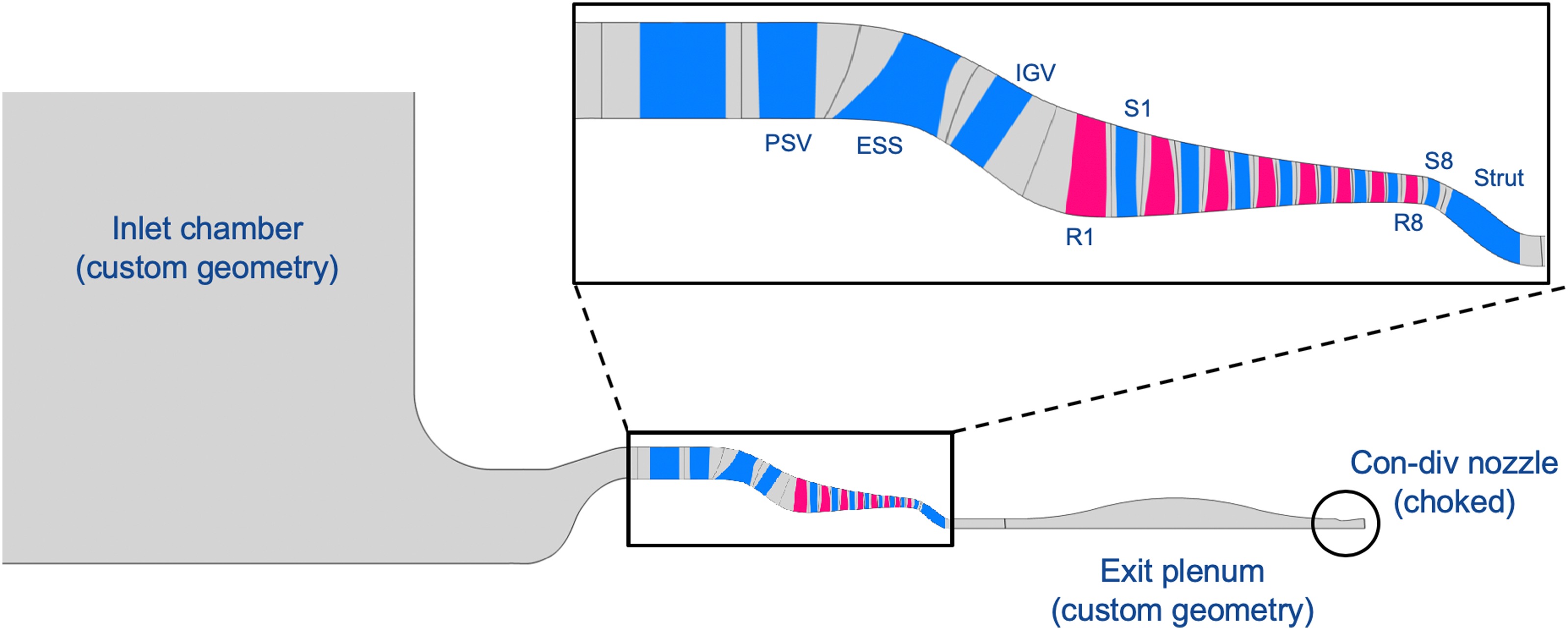
The geometry investigated in this paper is a modern, high-speed, 8-stage intermediate pressure compressor (IPC), representative of an existing rig (Dodds and Vadhati, 2015a) presented in Figure 2. High-fidelity, post-stall numerical simulations of this compressor have been carried out using AU3D at Imperial College, where deep surge cycles were simulated at part-speed (85% aero-speed) and design speed (100% aero-speed). The results for part-speed modelling have been reported in (Zhao et al., 2018) and the results for design speed are reported in (Zhao et al., 2020).
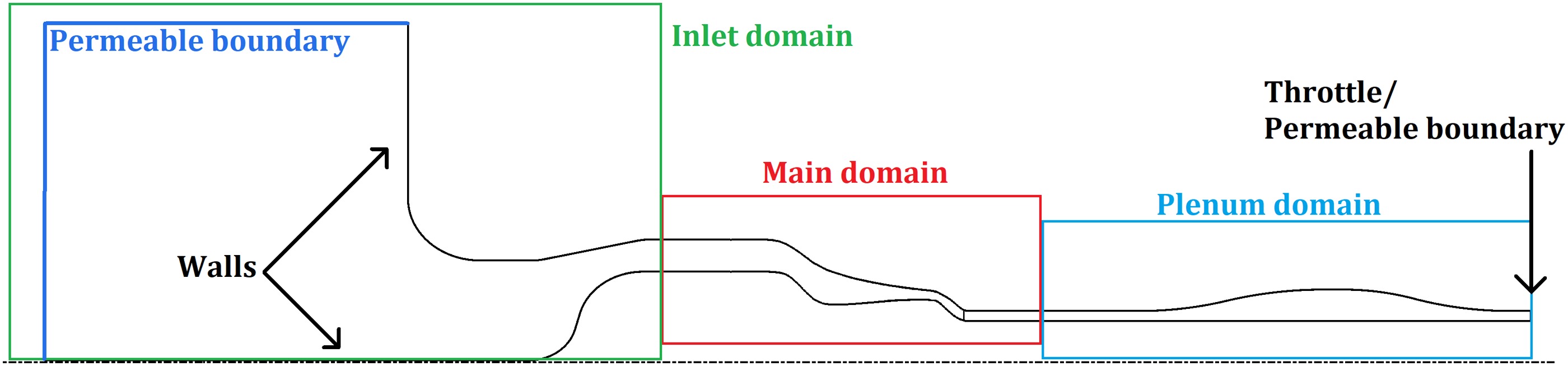
The ACRoSS model is formed by a main domain, an inlet domain used to reproduce the inlet chamber, and a throttled plenum, as in Figure 3. The main domain contains all the blade rows, including a row of struts, a row of pre-swirlers, and the ESS in front of the compressor and a row of struts downstream of the last stator. The compressor has a row of variable IGVs and 2 rows of VSVs, which have the same stagger angle settings as AU3D for both cases; these are custom settings and are different from the real schedule. No bleed valve, tip clearance or penny gap is considered. Only basic geometry data is required as input to ACRoSS. This includes the geometry in the meridional plane and the blade angles and maximum thickness at different positions in the span-wise direction. In all simulations ISA SLS (international standard atmosphere, sea level steady) conditions are applied at the far-field inlet boundaries while a low pressure is applied at the outlet to ensure the throttle remains choked during surge. Shaft speed is maintained constant during the simulations.
Figure 3.
Meridional view of the ACRoSS model of the 8-stage IPC test case; formed by an inlet and main domain, and an optional plenum domain.
The ACRoSS simulations are run with a meridional mesh of 2,500 axial X 7 radial elements in the main domain, 8,813 triangular elements in the inlet domain and 9,454 in the plenum domain. The grid is revolved around the axis to form 140 circumferential sectors, for a total of ∼5 million elements for the largest set-up. The same inlet domain is used in all the simulations presented in this paper, while the outlet set-up used is specified for each case. Surge simulations of the 100% speed case have been run with the number of elements in each direction multiplied by 1.5, and with the CFL condition halved to ensure that the surge cycles presented here are grid and time independent in terms of both performance and flow-field structures observed. For some of the simulations presented, a 2D version of ACRoSS is used. This is an axisymmetric simulation obtained by setting only one element in the circumferential direction.
The ACRoSS simulations are run on a HPC facility in Cranfield University on 40 CPUs with a computational cost of ∼5 days for 100 revolutions for the 85% corrected speed case with the largest number of elements. As a result, the longest simulation presented in this paper lasted ∼4 days. For comparison, the AU3D simulation for the 85% speed case has 300 million elements and requires one day per rotor revolution using 192 CPU.
Inlet/outlet domain modelling
ACRoSS contains an automatic mesh generator to create a structured uniform quadrilateral mesh; however, this has been designed for simple annuli and cannot be used to reproduce more complicate geometries like the inlet and plenum which are part of the AU3D model (see Figure 2).
A new capability has been added to the code to solve complex domains, symmetric to the main rotation axis, attached to the inlet and outlet of the main domain. The Euler solver has been adapted to work on a triangular mesh with an external boundary, solid walls, and an internal boundary interfaced with the main domain. For the present work, the triangular mesh has been created using ANSYS® MeshingTM (as contained in ANSYS® WorkbenchTM, Release 18.2). The mesh is then pre-processed and translated into a formatted input file for ACRoSS. The mesh supplied to the code is two-dimensional in the meridional plane and is made three-dimensional by revolution along the symmetry axis (see Figure 4).
Figure 4.
Example of three-dimensional inlet domain generated by rotation around the symmetry axis x (left) and plenum domain outlet boundary with variable throttle (right).

The existing version of the code uses a zero-dimensional adiabatic plenum model to set the static pressure at the domain outlet as proposed by Greitzer for stall simulation (Greitzer, 1976). The plenum is modelled as a volume with a single value of density and temperature discharging through the atmosphere with a convergent nozzle and is governed by the continuity and energy equations.
With the new capability introduced, a complex domain can be applied at the back of the main domain to reproduce the plenum volume; this allows to capture all the dynamics of the fluid contained in the plenum. However, it is necessary to introduce a method to throttle the domain and control the simulation. This was implemented in ACRoSS by introducing a dynamic change of the boundary conditions, which can be switched sequentially from permeable boundaries to solid wall, from the tip to the hub, as in Figure 4. The permeable boundaries of inlet and outlet domains are modelled using reflective boundary conditions. Total pressure and temperature are imposed on entering flows and static pressure is imposed on outgoing flows. When the 0D plenum model is employed, non-reflective boundary conditions are used at the main domain outlet.
Results and discussion
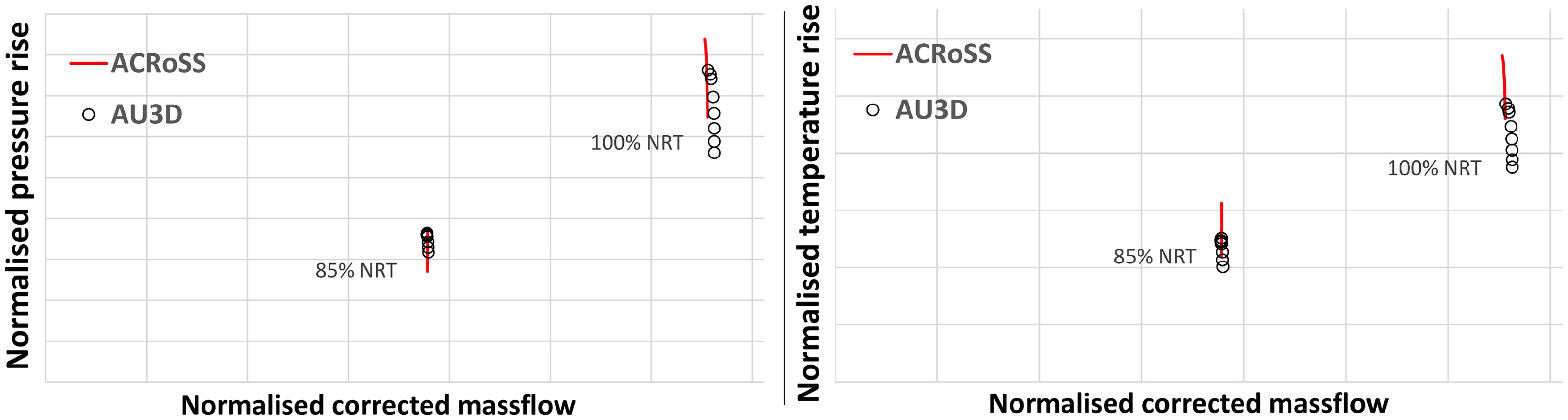
As a first step, the unstalled characteristics are generated using ACRoSS in 2D mode and compared with those generated by AU3D, as shown in Figure 5. The performance is presented in terms of corrected massflow, total pressure rise and total temperature rise, all normalised using the value in design conditions as reported by the manufacturer. The capacity of the compressor is matched within 5% for both speeds, while the temperature rise is always over-predicted by ACRoSS. The surge line is predicted very closely at 85% speed with the maximum pressure rise matching within 5%, but at design speed ACRoSS over-predicts the maximum pressure rise by ∼12%. In ACRoSS the stall is triggered by exceeding a minimum blade row velocity ratio predicted by the empirical correlations, which controls the maximum pressure rise. However this does not affect the performance during the post-stall transient and the higher maximum pressure rise has little effect on the matching of the initial flow reversal. Total temperature rise is over-predicted by ACRoSS by ∼13% in both cases. For the intends and purposes of this study, this level of matching between ACRoSS and AU3D at steady-state forward flow was deemed satisfactory and no further alignment between the 2 models was attempted.
85% speed surge case
The 85% corrected speed case is compared with the data from AU3D which has been presented in (Zhao et al., 2018).
The surge is triggered by gradually closing the throttle at a stable operating condition. The plenum used for this case is very large compared to the one used for the 100% speed case, therefore only the 0D model is used, as this is deemed to be an acceptable assumption. The throttle is closed by 1% increments until stall occurs and kept constant afterwards. The simulation is run until a full surge cycle is obtained and the time histories of massflow (non-corrected), total pressure and temperature are compared with the data from AU3D as shown in Figure 6. Massflow and pressure rise are normalised using the values at stall inception in AU3D.
Figure 6.
Comparison of transient event time histories during surge at 85% speed from ACRoSS and AU3D. Compressor map (a), massflow at IGV inlet (b), total pressure (c) and total temperature (d) at IGV inlet and stator 8 outlet.
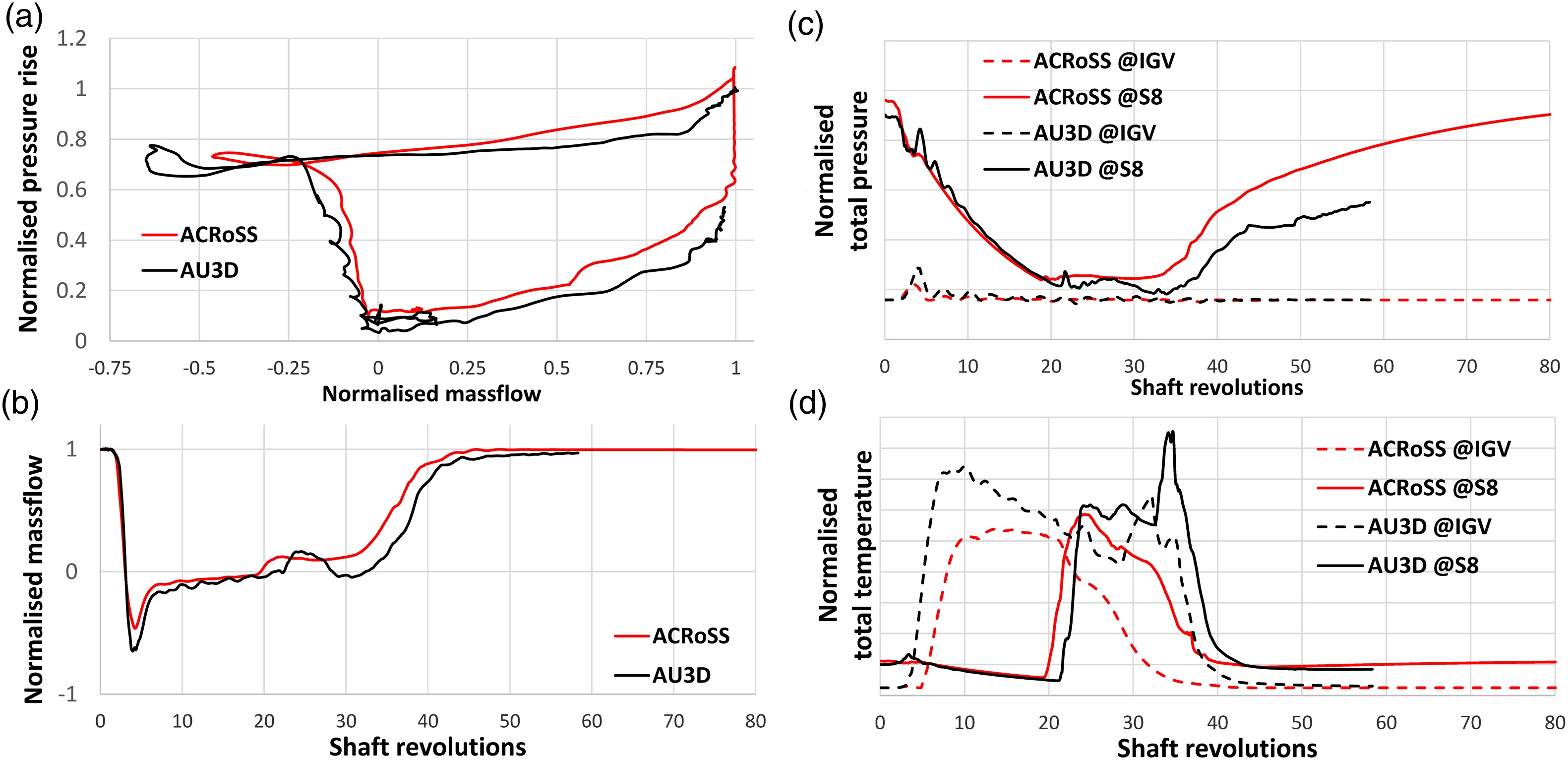
The reversal and blowdown parts of the map have a very close matching, with similar rates of pressure and massflow reduction (Figure 6b and c). During the blowdown some oscillations in pressure at stator 8 can be observed in AU3D, (Figure 6c); as it will be shown later, these are not modelled by ACRoSS because of the 0D plenum model. During the recovery part of the cycle AU3D predicts a temporary reduction and reversal of massflow during revolutions 25 to 35. This occurs as the hot air previously expelled into the inlet is re-ingested and, as the stages are filled with hot air >1,000 K, the compressor operates at very low corrected speed (less than 40% aero-speed). As the VSVs remain fixed at settings for 85% aero-speed, the compressor falls back into stall again. Recovery is achieved when the hot air is completely cleared from the compressor inlet (at around revolution 40). The ACRoSS simulation also predicts a similar reduction in massflow and delay in recovery, although the massflow does not cross
The temperature profiles in time are very similar, with a very good matching during specific instances of the transient event, Figure 6d. For example, the hot flow reaching the IGV (revolutions 5–8), the hot flow exiting through the last stage as the compressor recovers (revolutions 20–22), and the hot flow clearing the compressor as recovery is completed (revolutions 38–42). The magnitude of the temperature predicted by ACRoSS, however, is always smaller than the corresponding values from AU3D, this is observed also at 100% speed. As the thermodynamic model of gas is the same in both simulations, the authors suggest that the difference is caused by ACRoSS introducing a smaller turning force when operating in reverse/mixed flow. This is because ACRoSS represents separated flows as uniform and as such the flow momentum in these conditions is under-estimated, resulting in a smaller body-force to obtain the same turning and therefore less work introduced by the rotors.
100% speed surge case
The 100% corrected speed case is compared with data from AU3D. This surge event is triggered with the same method as previously. However, due to the higher pressure margin in ACRoSS, a slightly higher throttle closure is required compared to what was used in AU3D. The simulation is performed using both the 0D and the 3D plenum models to assess the effect of the different models. The simulations presented are labelled as:
ACRoSS/0D VOLUME: 3D inlet and main domain, 0D plenum model;
ACRoSS/3D VOLUME: 3D inlet and main domain, 3D plenum domain;
ACRoSS2D/2D VOLUME: 2D inlet and main domain, 2D plenum domain (axisymmetric).
About one and a half surge cycles from AU3D are available; the results from the ACRoSS simulations are aligned in time with the first instance of surge and presented in Figure 7. As in the previous case, massflow (non-corrected) and pressure rise are normalised using the values at stall inception in AU3D.
Figure 7.
Comparison of time histories during surge at 100% speed from AU3D and ACRoSS with different set-ups. Compressor map (a), massflow at IGV inlet (b), total pressure rise (c), and total temperature (d) at IGV inlet and stator 8 outlet.
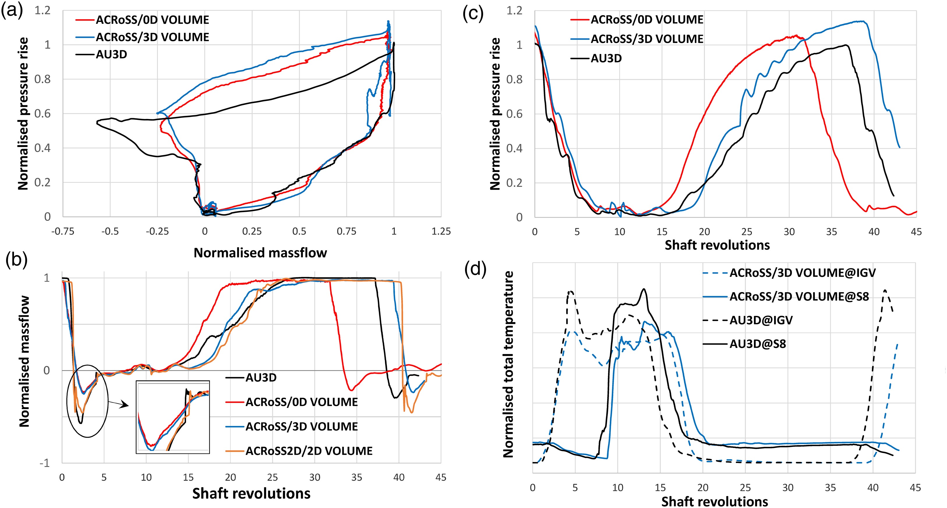
The two surges in AU3D simulations have different levels of asymmetry. To trigger the stall, the throttle is closed in a single step, which causes pressure waves to travel upstream. As mid stages are operating close to stall, a pressure wave causes one of the blade rows to separate in three passages simultaneously. Due to the multiple starting points, the first flow reversal occurs very fast and in a much more axisymmetric fashion, which results in higher maximum reverse flow as can be seen in Figure 7b at revolution 2.5. Without strong pressure waves instead, the second surge initiates as a growing 1-cell full-span rotating stall, gradually occupying the full annulus.
The ACRoSS 3D simulations predict a lower level of negative massflow during the first surge (revolution 2.5) and a similar level for the second surge (revolution 39–40). The reason for discrepancy is that in ACRoSS the stall inception is always very asymmetric, due to the random distortion forcing one circumferential position to stall first. Thus in ACRoSS stall inception presents a rotating stall growing to cover the whole annulus. To obtain a more axisymmetric surge, a 2D simulation was performed and compared to the first cycle of AU3D, as shown in Figure 7b. As it can be observed, the 2D version of ACRoSS closely matches the axisymmetric flow reversal at revolution 2.5, matching the rate of massflow reduction, the negative peak and in particular the step change in massflow highlighted in the zoomed view (this will be described in detail in the next section). Aside from the initial reversal, the 2D and 3D simulations show similar behaviour with an almost identical surge period. As in the part-speed case, after the initial recovery massflow reduces below zero temporarily when hot air is re-ingested at revolutions 10–13. This is closely reproduced by ACRoSS with all set-ups. Figure 7c presents a comparison of time history for static pressure rise. The oscillations during the recovery phase (and partly during the blowdown phase) which are observed in AU3D are re-produced by ACRoSS only when the 3D plenum is used. The use of a 3D plenum model in ACRoSS delays the recovery and gives a better matching in surge frequency; with the flow reaching the unstalled characteristic at about the same moment as AU3D at revolution 25. These results seem to indicate that the dynamics of the plenum, and the pressure waves it generates, have a non-negligible effect on the simulation. The re-pressurization in ACRoSS is faster but, as the compressor has a higher surge margin, it takes longer before the next surge cycle starts and the surge period is in fact ∼5% longer.
In Figure 7d the profile of temperature predicted by AU3D is compared to ACRoSS with the 3D outlet domain set-up. As in the previous simulation, the timing of the hot flow reaching the inlet and outlet is very similar but ACRoSS under-predicts the peaks of hot temperature.
Flow-field comparison
During surge some typical flow-field structures are observed in AU3D during specific parts of the cycle; in this section the flow-field during the 100% surge cycle is analysed to assess the capability of the low-order model to correctly reproduce them.
In AU3D, the stall inception of the second surge cycle occurs as a growing rotating stall cell; starting from a single point of reverse flow and gradually covering the whole annulus in less than 3 revolutions. This is presented in Figure 8 using the axial velocity at stator 4 exit at half span. The flow-field is analysed using the 3D version of ACRoSS in the same axial and radial position and the “boundaries” of the rotating stall cell are recorded (identified by the axial flow reversing,
Figure 8.
Axial velocity at stator 4 exit half span during stall inception as predicted by AU3D, with overlaid rotating stall boundaries as modelled by ACRoSS.

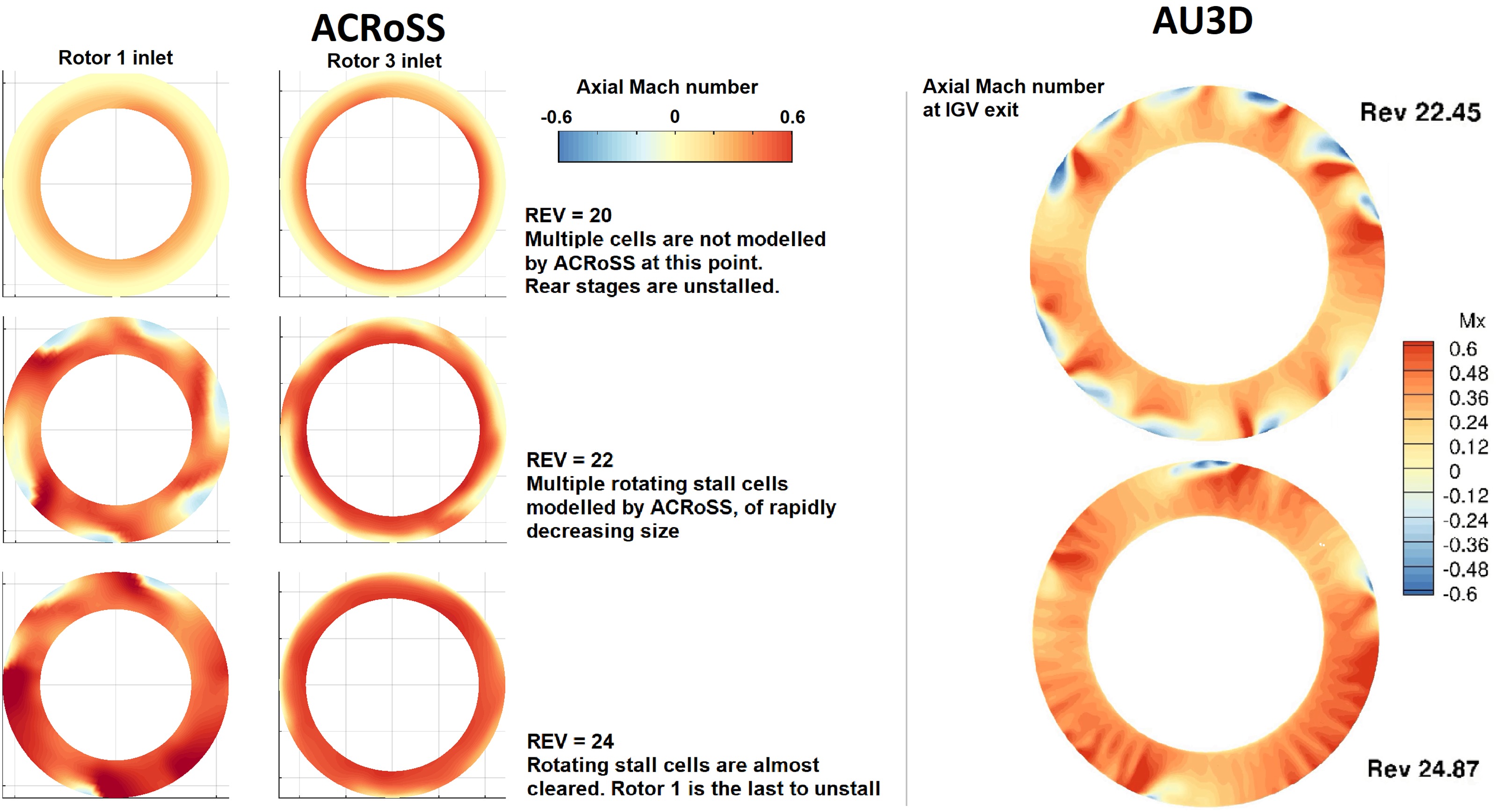
Rotating stall is also observed during the recovery phase of the surge cycle. In the 100% speed AU3D simulation, two distinctive types of rotating stall are observed: initially a higher-order low magnitude multi-stall cell is observed at revolutions 18–23, followed by a higher amplitude, half span 4-cell rotating stall which lasts from revolution 24 until recovery is completed, by which time the cell size reduces to zero. During this period the stall is confined to the front of the compressor and the last 4 stages are completely unstalled. The axial velocity profiles during the surge cycle as modelled by the 3D version of ACRoSS are presented for comparison in Figure 9. ACRoSS correctly reproduces the axial distribution of the stall, but does not model the initial part of rotating stall and remains in an axi-symmetric state. Only afterwards, at revolution 22, the reversed flow breaks up into a series of high-amplitude, rotating stall cells which reduce in size until recovery is completed, similarly to what is observed in the high-fidelity model.
Figure 9.
Mach number contours at different rotor inlets during recovery as modelled by ACRoSS (left) and axial Mach number contour at IGV exit from AU3D simulations (right).
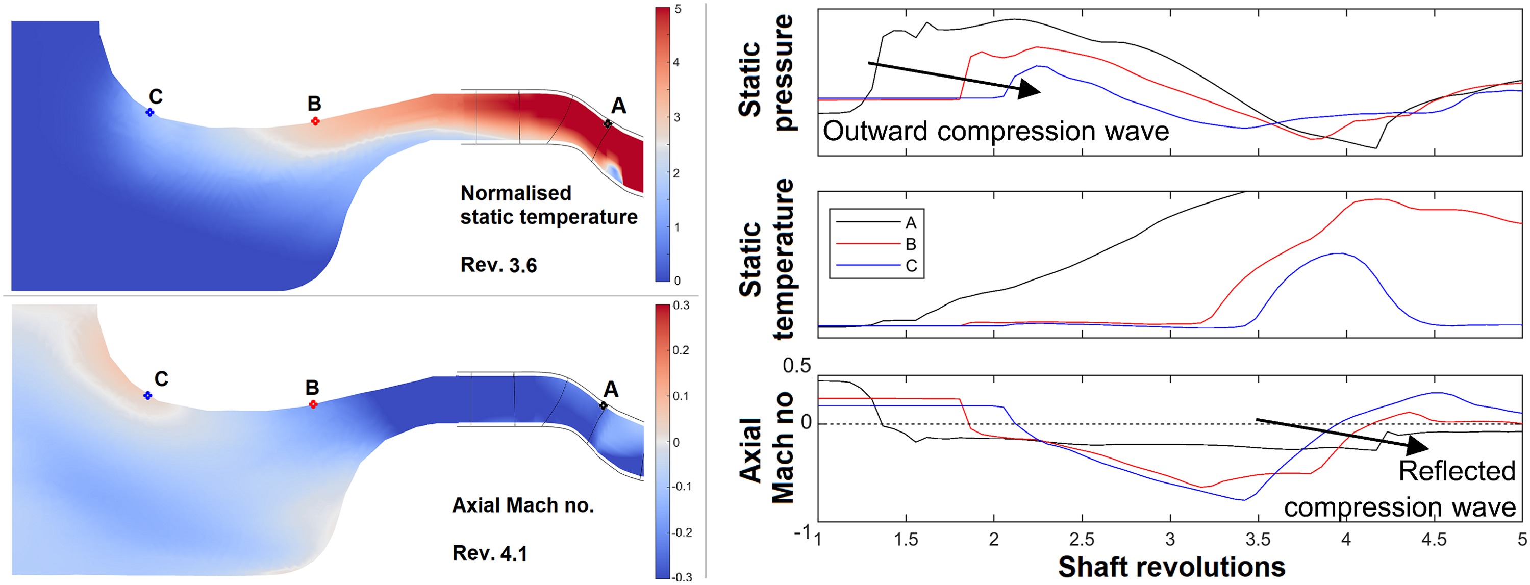
The profile of massflow at IGV inlet from AU3D shown in Figure 7b has a very distinctive jump at revolution 4.2. This was observed to be caused by a reflection of convected entropy wave at the opening in the inlet chamber. The inlet flow-field of a simulation using the 2D version of ACRoSS is investigated to detect the presence of the same mechanism.
Figure 10 presents the pressure, temperature and Mach number from ACRoSS calculations at the IGV inlet (point A) and at two more positions on the casing during surge, together with the flow-field at two relevant moments in time. At revolution 1.5 the compression wave caused by the surge propagates outwards from the compressor and reaches the three probes sequentially. As it passes, it locally reverses the flow without causing substantial temperature rise. At approximately revolution 3.5 the hot air (>1,000 K), generated inside the compressor due to the flow reversal, is convected by the flow and reaches the inlet opening (point C). The pressure distribution of the expanding flow has to change to adapt to the new temperature and this generates pressure waves going inwards and outwards. The “reflected” compression wave going towards the compressor causes the axial Mach number to increase, as can be observed at revolutions 3.5 to 4. The wave reaches the IGV inlet at rev 4.2 and causes the jump as observed in the massflow traces. This demonstrates that the interaction of the surge and the upstream geometry is correctly reproduced by the low-order model.
Conclusions
This paper presented the validation of low-order simulations of surge in multi-stage, high-speed, axial compressors using the through-flow code ACRoSS. Validation is obtained by reproducing existing high-fidelity URANS simulations of surge events run by Imperial College using the code AU3D and comparing the results. Two complete surge events were modelled at 85% and 100% corrected speed and massflow, pressure and temperature time histories were compared with ACRoSS demonstrating a reasonable level of accuracy. Further validation was obtained by analysing the flow-field structures observed during surge in AU3D and demonstrating that these are correctly reproduced by ACRoSS. The structure analysed were:
the growth of rotating stall during surge inception,
the transient presence of rotating stall cells during recovery,
the interaction of surge with the inlet geometry.
The through-flow code offers a large benefit in terms of computational cost compared to the high-fidelity 3D CFD. The simulations run with ACRoSS required approximately 1 day for 20 revolutions using 40 CPUs; for comparison, AU3D required 1 day for rotor revolution using 192 CPUs.
Nomenclature
Symbols
A
Element section area
Cp
Specific heat capacity at constant pressure
f,
Body force, body force vector
Internal Energy
H
Enthalpy
Massflow
M
Mach number
P
Pressure
r
Radius (r)
t
Time (s)
T
Temperature (K)
Source vector
u
Flow velocity (u)
V
Volume (m3)
Work exchanged
θ
Circumferential position
ρ
Density
Ω
Shaft rotation speed
Rigid rotation vector